Section 9. Graphs and Graph Algorithms

This section presents a comprehensive examination of graph data structures and foundational graph processing algorithms, spanning structural representations, systematic traversals, exhaustive route enumeration, and single-source shortest path optimization. The work explores core conceptual definitions—covering directed, undirected, and weighted graphs along with topological vertex attributes (degrees, in-degrees, out-degrees, and self-loops)—and evaluates the operational trade-offs between adjacency matrices and adjacency lists in dynamic JavaScript environments. A central emphasis is placed on algorithmic execution and formal visualization using DRAKON diagrams. The section delivers detailed trace models and comparative analyses between Depth-First Search (DFS) and Breadth-First Search (BFS). Furthermore, it introduces a modular recursive backtracking framework capable of discovering and evaluating all simple paths between candidate vertices under multi-criteria constraints (distance and price). Finally, the study analyzes the mechanics and step-by-step state relaxation of Dijkstra’s algorithm for weighted path optimization, providing complete algorithmic complexity assessments and an integrated visual reference framework.

9.1. General Information. Basic Terminology

This section discusses data structures such as graphs. In mathematics, a graph is a structure consisting of vertices (nodes) and edges (connections) that connect these vertices.

In general, graphs share many similarities with trees, and one can consider trees as a special case of graphs. However, the practical value of graphs in solving real-world problems is much greater. Many tasks can be reduced to considering a set of objects whose properties are described by the relationships between them.

Such objects include:

Electrical and electronic circuits
Printed circuit boards
Road maps
Aviation routes
Descriptions of structural constructions
Game states and logic

Among the tasks that can be solved using graphs are:

Finding the shortest path between two vertices
Solving the problem of maximum capacity of pipelines, road networks, or computer networks
Distributing N workers to perform M different types of work
Choosing the most efficient method of problem solving, among others.

Formally, a graph is denoted as G = (V, E), where V is the set of vertices and E is the set of edges connecting them.

Directed and Undirected Graphs

A graph as a data structure is defined by a set of vertices and a set of connections between them. Depending on whether these connections have direction, graphs are divided into two main types: undirected graphs and directed graphs.

Undirected Graphs

An undirected graph is a graph in which edges have no direction. An edge between vertices u and v represents only the fact that these two vertices are connected. In other words, the connection u — v is equivalent to the connection v — u.

Formally, an undirected graph can be written as:

G = (V, E)

where V is the set of vertices and E is the set of edges. Each edge connects two vertices.

The degree of a vertex v, denoted as deg(v), is the number of edges incident to v, that is, the number of edges connected to this vertex.

If loops are allowed, then a loop in an undirected graph contributes 2 to the degree of the vertex.

This is because a loop has two endpoints, and both endpoints are incident to the same vertex.

For example, if a vertex v has one ordinary edge connected to another vertex and one loop, then:

deg(v) = 1 + 2 = 3

Directed Graphs

A directed graph, or digraph, is a graph in which every edge has a direction. Directed edges are often called arcs.

An arc from vertex u to vertex v is written as:

(u, v)

and represents a connection directed from u to v.

Unlike in an undirected graph, the arcs (u, v) and (v, u) are different connections.

For directed graphs, the degree of a vertex is divided into two separate characteristics:

The in-degree of a vertex v, denoted as deg^-(v), is the number of arcs entering v.
The out-degree of a vertex v, denoted as deg^+(v), is the number of arcs leaving v.

The total degree of a vertex in a directed graph is the sum of its in-degree and out-degree:

deg(v) = deg^-(v) + deg^+(v)

If a directed graph contains a loop (v, v), then this loop both enters and leaves the same vertex v. Therefore, it increases the in-degree by 1 and the out-degree by 1:

deg^-(v) += 1
deg^+(v) += 1

As a result, a loop increases the total degree of the vertex by 2.

In short, an undirected edge represents a symmetric connection between two vertices, while a directed edge represents an ordered connection. For this reason, directed graphs distinguish between incoming and outgoing arcs.

Figure 9.1. Graphical representation of (a) an undirected graph; (b) a directed graph (digraph)

Adjacency, Incidence, and Degree

A vertex and an edge are incident if the vertex is one of the endpoints of the edge.

Refined Terms for Directed Graphs (Digraphs):

In-degree (deg^-(v)): The number of edges directed into the vertex. In flow-based models, this represents the "input" capacity.
Out-degree (deg^+(v)): The number of edges directed away from the vertex. In state machines, this represents the number of possible state transitions.
Total Degree: The sum of in-degree and out-degree.
Self-Loop (Digraph): A special case where an edge starts and ends at the same vertex. It contributes exactly 1 to the in-degree and exactly 1 to the out-degree.

Figure 9.2. Basic graph parameters and node dimensions

9.2. Graph Representation Methods

Solving problems related to processing a data set organized in the form of graphs requires modeling them in computer programs. In practice, two structures are typically used to model the structure of a graph: the adjacency matrix and the adjacency list.

Adjacency Matrix

An adjacency matrix is a two-dimensional array that indicates the existence of a relationship between two vertices. If the graph has V vertices, then the adjacency matrix is a V × V array. In an undirected graph, the adjacency relationship is symmetric: if vertex u is adjacent to v, then v is also adjacent to u. This symmetry is reflected in the adjacency matrix, which is always symmetric about its main diagonal.

In contrast, for a directed graph (or digraph), the relationship is not necessarily symmetric. An edge (u, v) means vertex v is adjacent from vertex u, and this is indicated in the matrix by a '1' at position A[u][v] only.

Figure 9.3. Adjacency matrix layout for undirected and directed graphs

Adjacency List

In some cases, a more memory-efficient way to represent a graph is to use an adjacency list. This method involves an array of linked lists (or nested arrays), where each individual list contains information about which vertices are adjacent to a given one.

Figure 9.4. Adjacency list structural representation

Comparison and Complexity

The space complexity of representing a graph depends heavily on the chosen data structure:

Adjacency Matrix: Requires O(V^2) memory. This is memory-intensive, especially for large, sparse graphs (graphs with relatively few edges). It also often requires knowing the number of vertices in advance.
Adjacency List: Requires O(V + E) memory, where E is the number of edges. This is much more efficient for sparse graphs, which are common in real-world applications.

In practice, the choice between these representations is a trade-off. An adjacency matrix is often preferable for dense graphs (graphs where the number of edges approaches V^2) and when frequent edge lookups are required (O(1) complexity). An adjacency list is generally better for sparse graphs.

Weighted Graphs

Many real-life problems require modeling graphs with numerical values associated with edges, such as distance, cost, or travel time. Such graphs are called weighted graphs. In an adjacency matrix, the weight is stored as the value of the matrix element (instead of '1'), and a special value (like ∞ or 0) can represent the absence of an edge. In an adjacency list, each element in the list is typically a structure containing both the adjacent vertex ID and the edge weight.

Figure 9.5. Adjacency list equipped with a 'weight' field

Graph Representation in JavaScript

Since JavaScript is a dynamic language, we rely on the flexibility of Objects, Arrays, and built-in collections.

Adjacency Matrix in JavaScript

// Initialize a 3x3 matrix for an undirected graph
const numVertices = 3;
const adjMatrix = Array(numVertices).fill().map(() => Array(numVertices).fill(0));

function addEdgeMatrix(u, v) {
    adjMatrix[u][v] = 1;
    adjMatrix[v][u] = 1; // For undirected graph
}

addEdgeMatrix(0, 1);
addEdgeMatrix(1, 2);

// Check adjacency (O(1))
console.log(adjMatrix[0][1]); // 1

Adjacency List in JavaScript

const numVertices = 3;
const adjList = Array(numVertices).fill().map(() => []);

function addEdgeList(u, v) {
    adjList[u].push(v);
    adjList[v].push(u); // For undirected graph
}

addEdgeList(0, 1);
addEdgeList(1, 2);

// Check adjacency (O(degree(u)))
console.log(adjList[0].includes(1)); // true

Weighted Graph in JavaScript

const weightedAdjList = Array(numVertices).fill().map(() => []);

function addWeightedEdge(u, v, weight) {
    weightedAdjList[u].push({ node: v, weight });
    weightedAdjList[v].push({ node: u, weight }); // For undirected weighted graph
}

addWeightedEdge(0, 1, 5);
addWeightedEdge(1, 2, 10);

9.3. Fundamentals of Graph Traversal

Once a graph structure is established, the next logical task is to systematically visit all its vertices. This process is called graph traversal. There are two primary techniques: Depth-First Search (DFS) and Breadth-First Search (BFS).

The fundamental difference between DFS and BFS lies in the order in which they explore the graph, which stems from the underlying data structure they use to manage yet-to-be-visited vertices:

Depth-First Search (DFS) uses a stack (often implemented via recursion or explicit arrays) to explore as deep as possible along each branch before backtracking. While DFS does not inherently find shortest paths, it is indispensable for tasks like detecting cycles, topological sorting, and exploring a graph when its overall structure is not known in advance.
Breadth-First Search (BFS) uses a queue to explore the graph level by level. It visits all direct neighbors of the starting vertex, then all of their neighbors, and so on. BFS is guaranteed to find the shortest path (in terms of the number of edges) in an unweighted graph.

The step-by-step process for each algorithm is shown in the tables below for the example graph, starting from vertex V₀.

Figure 9.6. Reference directed graph for demonstrating DFS and BFS traversals

Depth-First Search (DFS) — Using Stack (LIFO)

Table 1. Detailed DFS Trace Table from Vertex `V₀`
Step	Action	Current Vertex	Unvisited Neighbors	Stack Content (LIFO)	Visited Order
1	Initialization Push the start vertex onto the stack.	0	`[1, 3]` ([Both neighbors are unvisited. Due to the reverse `i--` loop in your chart, they are pushed onto the stack as `[3, 1]`})	`[3, 1]`	`[0]`
2	Pop from stack Extract the last element of the stack.	1	`[2]` ([The only outgoing neighbor of vertex 1])	`[3, 2]` (Vertex `V₂` is pushed on top of vertex 3)	`[0, 1]`
3	Pop from stack Extract vertex `V₂`.	2	`[]` ([Vertex `V₂` is an absolute dead-end; it has no outgoing edges])	`[3]` (The stack shrinks; no new elements are added)	`[0, 1, 2]`
4	Pop from stack Extract vertex `V₃`.	3	`[4, 5]` _([Vertex `V₃` has three neighbors: `[2, 4, 5]`. `V₂` is already visited, only `[5, 4]` are pushed in reverse order])	`[5, 4]`	`[0, 1, 2, 3]`
5	Pop from stack Extract vertex `V₄`.	4	`[]` ([Vertex `V₄` has no outgoing edges])	`[5]`	`[0, 1, 2, 3, 4]`
6	Pop from stack Extract vertex `V₅`.	5	`[6]` ([Vertex `V₅` has two neighbors: `[4, 6]`. Since `V₄` was already visited in step 5, only vertex `V₆` is pushed])	`[6]`	`[0, 1, 2, 3, 4, 5]`
7	Pop from stack Extract the final vertex.	6	`[]` ([Vertex `V₆` has no outgoing edges])	`[]` (The stack is completely empty)	`[0, 1, 2, 3, 4, 5, 6]`
8	Termination The condition `stack.length > 0` returns `No`. Exit loop.	—	—	`[]`	Final Result: `[0, 1, 2, 3, 4, 5, 6]`

Key Principle of DFS: The stack operates on the LIFO (Last In, First Out) principle. The algorithm dives deep into the structural branches before backtracking.

Breadth-First Search (BFS) — Using Queue (FIFO)

Table 2. Detailed BFS Trace Table from Vertex `V₀`
Step	Action	Current Vertex	Unvisited Neighbors	Queue Content (FIFO)	Visited Order
1	Initialization Enqueue the start vertex.	0	`[1, 3]` ([Both neighbors are unvisited. Due to the direct `i++` loop in your chart, they are enqueued as `[1, 3]`})	`[1, 3]`	`[0]`
2	Dequeue (Shift) Extract the first element from the queue head.	1	`[2]` ([The only outgoing neighbor of vertex 1])	`[3, 2]` (Vertex `V₂` is appended to the tail of the queue)	`[0, 1]`
3	Dequeue (Shift) Extract vertex `V₃` from the queue head.	3	`[4, 5]` ([Vertex `V₃` has neighbors `[2, 4, 5]`. Vertex `V₂` is skipped as it is already in the queue. Only `[4, 5]` are appended])	`[2, 4, 5]`	`[0, 1, 3]`
4	Dequeue (Shift) Extract vertex `V₂`.	2	`[]` ([Vertex `V₂` has no outgoing edges])	`[4, 5]` (The queue shrinks from the front)	`[0, 1, 3, 2]`
5	Dequeue (Shift) Extract vertex `V₄`.	4	`[]` ([Vertex `V₄` has no outgoing edges])	`[5]`	`[0, 1, 3, 2, 4]`
6	Dequeue (Shift) Extract vertex `V₅`.	5	`[6]` ([Vertex `V₅` has neighbors `[4, 6]`. Vertex `V₄` is skipped as it is already visited. Only vertex `V₆` is appended])	`[6]`	`[0, 1, 3, 2, 4, 5]`
7	Dequeue (Shift) Extract the final vertex.	6	`[]` ([Vertex `V₆` has no outgoing edges])	`[]` (The queue is completely empty)	`[0, 1, 3, 2, 4, 5, 6]`
8	Termination The condition `queue.length > 0` returns `No`. Exit loop.	—	—	`[]`	Final Result: `[0, 1, 3, 2, 4, 5, 6]`

Key Principle of BFS: The queue operates on the FIFO (First In, First Out) principle. The algorithm expands outwards like a wave — evaluating immediate neighbors before expanding deeper.

Comparison: Stack vs. Queue

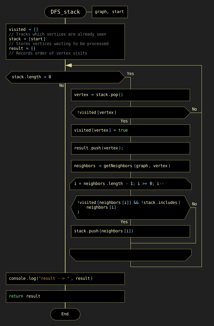
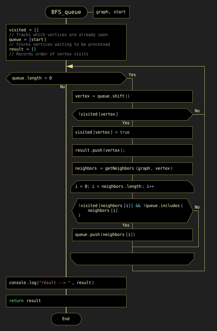
The comparison of traversal paths clearly illustrates the fundamental difference between the two traversal strategies. DFS, using a stack, delves deep into the graph’s branches, while BFS, using a queue, explores level by level ( (Figure 9.7).

Figure 9.7. Comparison of DFS and BFS traversal orders from vertex 0

Feature DFS (Stack) BFS (Queue)

Feature	DFS (Stack)	BFS (Queue)
Data Structure	Stack (LIFO)	Queue (FIFO)
Traversal Order From `V~~`	0 → 1 → 2 → 3 → 4 → 5 → 6	0 → 1 → 3 → 2 → 4 → 5 → 6
Strategy	"Depth-first" — explores branches completely	"Breadth-first" — explores level by level
Target Applications	Cycle detection, Topological sort	Shortest path in unweighted networks

Data Structure

Stack (LIFO)

Queue (FIFO)

Traversal Order From V~~

0 → 1 → 2 → 3 → 4 → 5 → 6

0 → 1 → 3 → 2 → 4 → 5 → 6

Strategy

"Depth-first" — explores branches completely

"Breadth-first" — explores level by level

Target Applications

Cycle detection, Topological sort

Shortest path in unweighted networks

DRAKON-Diagrams for DFS and BFS

Before analyzing the practical considerations for selecting an appropriate traversal strategy, it is instructive to examine the algorithmic logic encoded in the implementation. The Drakon-diagrams below provide a visual representation of the control flow for both Depth-First Search (DFS) and Breadth-First Search (BFS) algorithms.

These diagrams decompose the traversal process into discrete decision points and operations, illustrating how the choice of underlying data structure — a stack for DFS versus a queue for BFS — fundamentally shapes the execution path.

Figure 9.8a. Drakon-diagram illustrating the control flow of DFS (Depth-First Search)

Figure 9.8b. Drakon-diagram illustrating the control flow of BFS (Breadth-First Search)

Choosing Between DFS and BFS

In practice, the choice between DFS and BFS depends on the specific problem requirements:

Task	Recommended Algorithm	Reason
Shortest path (unweighted)	BFS	Guarantees minimum number of traversed edges
Graph connectivity	DFS or BFS	Any systematic traversal satisfies this criteria
Cycle detection	DFS	Highly efficient with tracking backtracking state
Topological sorting	DFS	Resolves dependencies naturally via post-order tracking

Task

Recommended Algorithm

Reason

Shortest path (unweighted)

BFS

Guarantees minimum number of traversed edges

Graph connectivity

DFS or BFS

Any systematic traversal satisfies this criteria

Cycle detection

DFS

Highly efficient with tracking backtracking state

Topological sorting

DFS

Resolves dependencies naturally via post-order tracking

9.4. Calculation of Paths and Travel Costs Between Two Vertices

This subsection examines the problem of finding all possible simple routes between two vertices in a weighted graph. For each route, the algorithm calculates two cumulative characteristics:

total distance, measured in kilometers;
total travel price, measured in arbitrary units.

The considered task differs from ordinary graph traversal. Classical BFS and DFS are usually used to determine the order of visiting vertices or to find one suitable path. In contrast, the algorithm described here enumerates all possible simple paths from a source vertex to a target vertex and evaluates each of them according to its accumulated weights.

This makes it possible to solve the following practical tasks:

find all possible routes between two selected vertices;
calculate the total distance of each route;
calculate the total travel price of each route;
compare routes according to different optimization criteria;
select the shortest, cheapest, or otherwise preferable route.

General Idea of the Algorithm

The algorithm is based on recursive backtracking. During the search, the program gradually constructs the current path from the source vertex to the target vertex. At each step, it selects one of the neighboring vertices, adds the corresponding edge characteristics to the accumulated sums, and continues the search recursively.

If the target vertex is reached, the current route is saved as a completed path. After that, the algorithm returns to the previous vertex, restores the former state, and tries another possible continuation.

Thus, the algorithm consists of two alternating phases:

forward movement to a neighboring vertex;
backward restoration of the previous state.

This mechanism makes it possible to enumerate all simple paths without revisiting vertices already included in the current route.

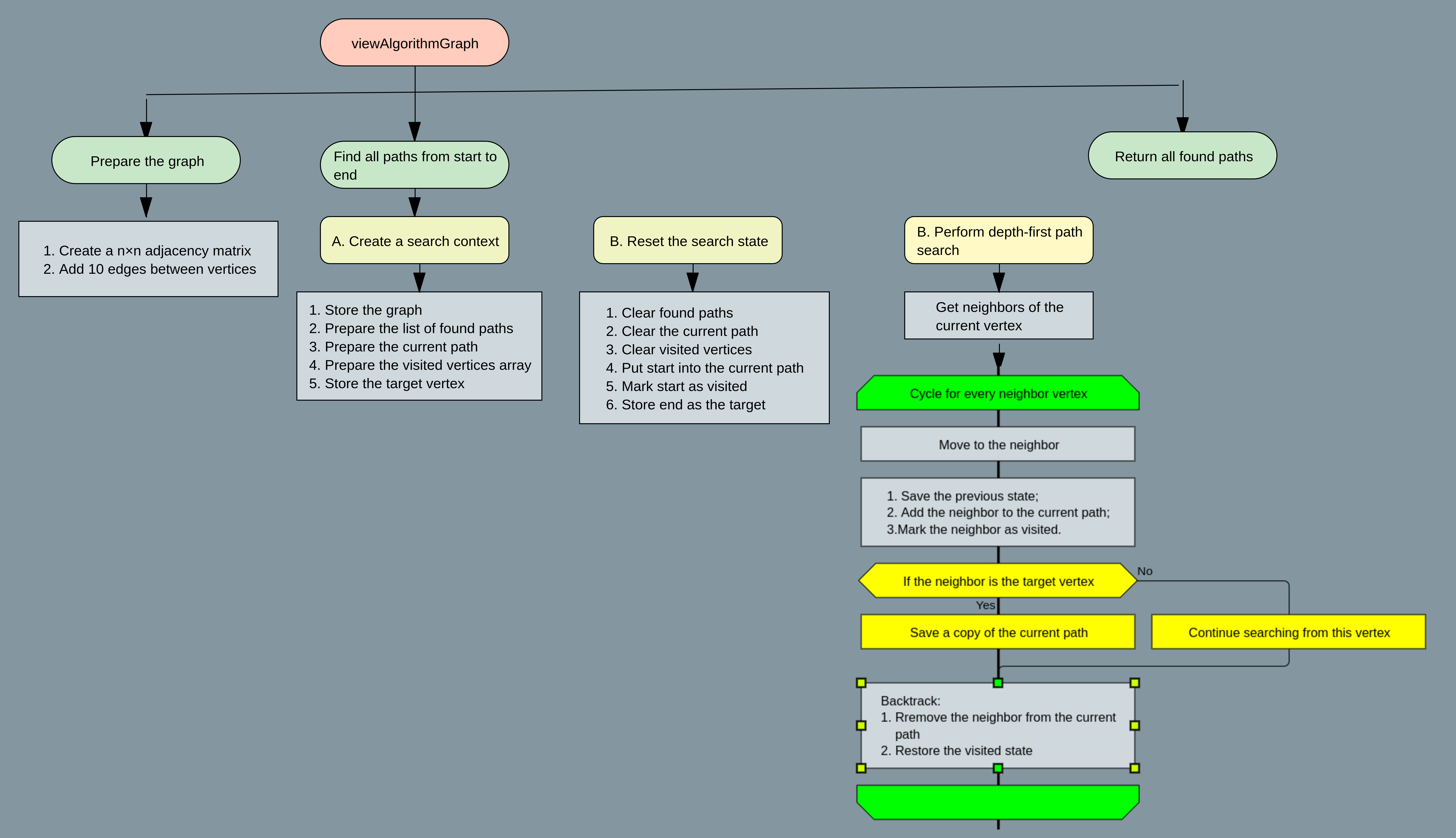
The overall structure of the functions involved in the path search is shown in Figure 9.9.

Figure 9.9. Mind map of path search functions

Functional Structure of the Path Search Module

The path search module is organized as a small group of cooperating functions. Each function performs a clearly separated role in the general recursive process.

The main control function is initPathSearch(). It prepares the initial search context and starts recursion.

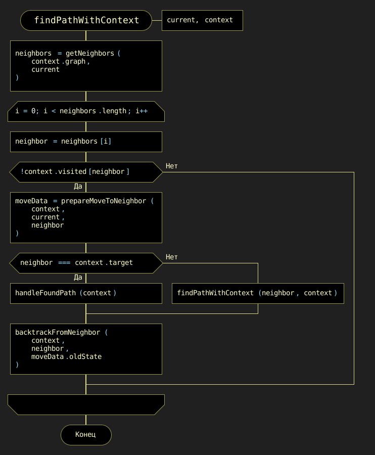
The recursive enumeration itself is performed by findPathWithContext(). This function checks the current vertex, processes its neighbors, and controls the transition from one vertex to another.

When the target vertex is reached, the function handleFoundPath() creates a structured description of the completed route and stores it in the resulting collection.

Two auxiliary functions support the backtracking mechanism:

prepareMoveToNeighbor() prepares the transition to a neighboring vertex and saves the current state;
backtrackFromNeighbor() restores the previous state after the recursive call has finished.

This functional decomposition separates the logic of initialization, recursive search, result processing, forward movement, and backward restoration.

Description of Key Functions

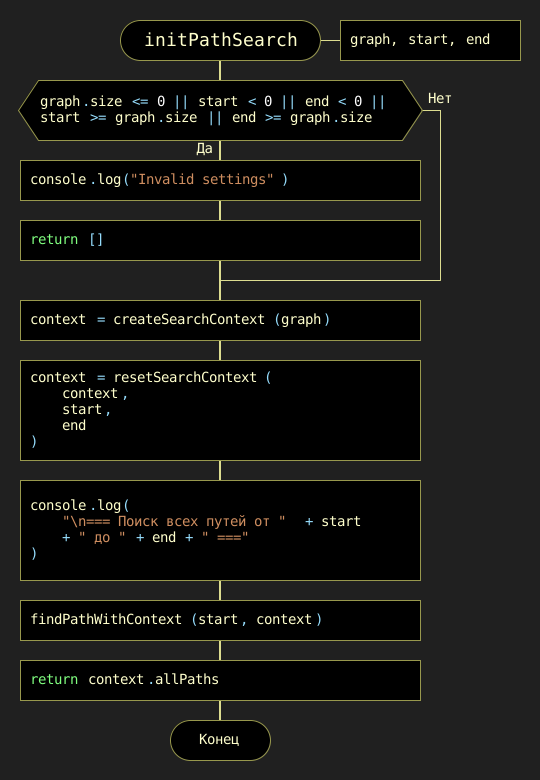
initPathSearch(graph, source, target)

The function initPathSearch() is the entry point of the path search module. It creates the search context, initializes all necessary data structures, and starts the recursive traversal of the graph.

Attribute Description

Attribute	Description
Purpose	Initializes the search for all paths from the source vertex to the target vertex. Creates the search context, resets accumulated parameters, and starts recursive graph traversal.
Parameters	`graph` — graph object containing the adjacency matrix and edge weights. `source` — identifier of the source vertex. `target` — identifier of the target vertex.
Return Value	Array `allPaths` containing all discovered paths as `pathInfo` objects.

Purpose

Initializes the search for all paths from the source vertex to the target vertex. Creates the search context, resets accumulated parameters, and starts recursive graph traversal.

Parameters

graph — graph object containing the adjacency matrix and edge weights.

source — identifier of the source vertex.

target — identifier of the target vertex.

Return Value

Array allPaths containing all discovered paths as pathInfo objects.

The initialization logic is shown in Figure 9.10.

Figure 9.10. DRAKON-diagram of the initialization function for path search

findPathWithContext(current, context)

The function findPathWithContext() is the core recursive function of the algorithm. It analyzes the current vertex and determines whether the target vertex has already been reached.

If the current vertex is the target, the completed path is processed by handleFoundPath(). Otherwise, the function checks all neighboring vertices and recursively continues the search through those neighbors that have not yet been visited in the current path.

Attribute Description

Attribute	Description
Purpose	Performs recursive enumeration of all possible simple paths from the current vertex to the target vertex. Updates the current path, accumulated distance, and accumulated price.
Parameters	`current` — identifier of the current vertex. `context` — search state object containing `target`, `graph`, `currentPath`, `totalDistance`, `totalPrice`, `visited`, and `allPaths`.
Return Value	`void`. The results are accumulated in `context.allPaths`.

Purpose

Performs recursive enumeration of all possible simple paths from the current vertex to the target vertex. Updates the current path, accumulated distance, and accumulated price.

Parameters

current — identifier of the current vertex.

context — search state object containing target, graph, currentPath, totalDistance, totalPrice, visited, and allPaths.

Return Value

void. The results are accumulated in context.allPaths.

The recursive search logic is shown in Figure 9.11.

Figure 9.11. DRAKON diagram of the recursive path search function

handleFoundPath(context)

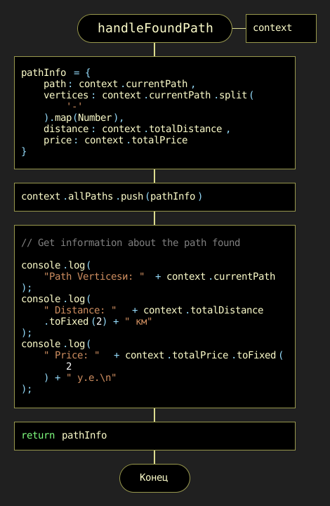
The function handleFoundPath() is called when the recursive search reaches the target vertex. At this moment, the current route is complete and can be transformed into a structured result.

The function creates a pathInfo object that contains the route itself, the list of vertices, total distance, and total price. This object is then added to the collection of found paths.

Attribute Description

Attribute	Description
Purpose	Creates and stores a structured record of a completed path from the source vertex to the target vertex.
Parameters	`context` — search state object containing `currentPath`, `totalDistance`, `totalPrice`, and `allPaths`.
Return Value	`pathInfo` object with the fields `path`, `vertices`, `distance`, and `price`.

Purpose

Creates and stores a structured record of a completed path from the source vertex to the target vertex.

Parameters

context — search state object containing currentPath, totalDistance, totalPrice, and allPaths.

Return Value

pathInfo object with the fields path, vertices, distance, and price.

The path handling logic is shown in Figure 9.12.

Figure 9.12. DRAKON diagram of the Path Handler function

prepareMoveToNeighbor(context, current, neighbor)

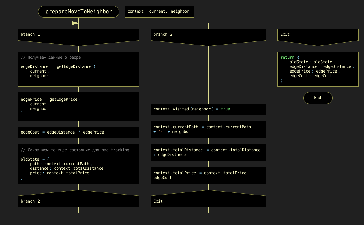
The function prepareMoveToNeighbor() prepares the forward movement from the current vertex to one of its neighbors. It reads the edge characteristics, updates the current path, increases the accumulated distance and price, and marks the neighbor as visited.

Before changing the context, the function saves the previous state. This saved state is required later for correct backtracking.

Attribute Description

Attribute	Description
Purpose	Prepares transition to a neighboring vertex and saves the previous state of the search context.
Parameters	`context` — search state object. `current` — identifier of the current vertex. `neighbor` — identifier of the neighboring vertex.
Return Value	`oldState` object containing the previous values of `currentPath`, `totalDistance`, and `totalPrice`.

Purpose

Prepares transition to a neighboring vertex and saves the previous state of the search context.

Parameters

context — search state object.

current — identifier of the current vertex.

neighbor — identifier of the neighboring vertex.

Return Value

oldState object containing the previous values of currentPath, totalDistance, and totalPrice.

The transition preparation logic is shown in Figure 9.13.

Figure 9.13. DRAKON diagram of the Transition Preparation function

Reversing function `backtrackFromNeighbor(context, neighbor, oldState)`

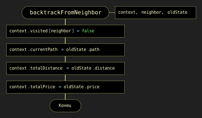
The function backtrackFromNeighbor() performs the reverse phase of the algorithm. After the recursive processing of a neighboring vertex is completed, the algorithm must return to the previous state in order to try another possible route.

This function clears the visited flag for the processed neighbor and restores the path, distance, and price values saved in oldState.

Attribute Description

Attribute	Description
Purpose	Restores the previous search state after processing a neighboring vertex. This enables exhaustive enumeration of alternative routes.
Parameters	`context` — search state object. `neighbor` — vertex whose processing has been completed. `oldState` — object containing the previous values of `currentPath`, `totalDistance`, and `totalPrice`.
Return Value	`void`. The search context is restored to the previous state.

Purpose

Restores the previous search state after processing a neighboring vertex. This enables exhaustive enumeration of alternative routes.

Parameters

context — search state object.

neighbor — vertex whose processing has been completed.

oldState — object containing the previous values of currentPath, totalDistance, and totalPrice.

Return Value

void. The search context is restored to the previous state.

The backtracking logic is shown in Figure 9.14.

Figure 9.14. DRAKON diagram of the Backtracking function

Algorithmic Complexity Analysis

The implemented algorithm enumerates all simple paths between two vertices. Therefore, its running time may grow exponentially with the number of vertices.

In the worst case, especially for a dense graph, the number of possible simple paths can be very large. For this reason, the time complexity can be estimated as factorial or exponential, depending on the graph structure. A conservative upper estimate is:

\$O(V!)\$

where V is the number of vertices.

The space complexity is mainly determined by the recursion depth, the current path, and the visited array. Since a simple path cannot contain more than V vertices, the auxiliary space complexity is:

\$O(V)\$

This approach is suitable for small and medium-sized educational examples. However, for large dense graphs, exhaustive path enumeration becomes impractical. In such cases, specialized algorithms should be used depending on the optimization criterion, for example shortest path algorithms.

Program Execution Example

Using the example graph shown in Figure 9.15, the algorithm can find all simple paths from vertex 0 to vertex 5. Each path is represented as a sequence of vertices, along with the total distance and price calculated based on the edge weights.

Figure 9.15. Graphical representation of the path search process from vertex 0 to vertex 5

The following fragment shows an example of output for paths from vertex 0 to vertex 5.

// === Find all paths from 0 to 5 ===
//
// Path Vertices: 0-1-4-3-5
// Distance: 101.28 km
// Price: 31.80 u.
//
// Path Vertices: 0-6-3-5
// Distance: 94.21 km
// Price: 21.60 u.

The first route has a greater distance and price. The second route is shorter and cheaper in this example. Therefore, the same set of found paths can be analyzed according to several criteria: minimum distance, minimum price, or a combined route quality indicator.

Summary

The developed module demonstrates how recursive backtracking can be applied to weighted graphs. Unlike simple traversal algorithms, this approach does not stop after finding one path. Instead, it systematically enumerates all possible simple paths from the source vertex to the target vertex and calculates the quantitative characteristics of each route.

This makes the module useful as an educational example for understanding:

recursive graph traversal;
path construction;
state saving and restoration;
backtracking;
analysis of weighted routes;
comparison of alternative paths.

The same idea can be used as a basis for studying transportation logistics, route planning, and optimization problems.

9.5. Dijkstra’s Algorithm

Dijkstra’s algorithm is designed to find the shortest paths from a given start vertex to all other vertices in a weighted graph, provided that all edge weights are non-negative. This condition is essential: Dijkstra’s algorithm works correctly only when every edge weight is greater than or equal to zero.

The algorithm is named after the renowned Dutch computer scientist Edsger W. Dijkstra, who first conceived it in 1956. Today, Dijkstra’s algorithm is widely used in science, engineering, and everyday applications:

GPS navigation systems: finding the fastest routes while taking into account distances and traffic conditions.
Telecommunications networks: determining optimal paths for data routing, for example in OSPF and IS-IS protocols.
Robotics and games: real-time path planning and object navigation through maps.

Graph Representation for Dijkstra’s Algorithm

For our demonstration of Dijkstra’s algorithm, we will use the graph shown in Figure 9.16. This graph consists of six vertices, labeled from 0 to 5, connected by weighted edges.

Figure 9.16. Target topology setup for Dijkstra shortest path calculation

In JavaScript, this weighted graph can be represented as an object whose keys are vertices and whose values describe adjacent vertices and edge weights:

const graph = {
    0: { 1: 48.3, 2: 40.7, 5: 25.4 },
    1: { 0: 48.3, 2: 37.5, 3: 29.8 },
    2: { 0: 40.7, 1: 37.5, 3: 34.9, 5: 29.8 },
    3: { 1: 29.8, 2: 34.9, 4: 25.4 },
    4: { 3: 25.4, 5: 34.9 },
    5: { 0: 25.4, 2: 29.8, 4: 34.9 }
};

This representation corresponds to an undirected weighted graph. For example, the edge between vertices 0 and 1 has weight 48.3, and therefore it appears in both directions:

0: { 1: 48.3, ... }
1: { 0: 48.3, ... }

How the Algorithm Works

Dijkstra’s algorithm is based on a simple but powerful principle: it iteratively builds the set of vertices for which the shortest distance from the start vertex is already known, and uses these vertices to improve the distance estimates for the remaining vertices.

The mind map of Dijkstra’s algorithm is presented in Figure 9.17.

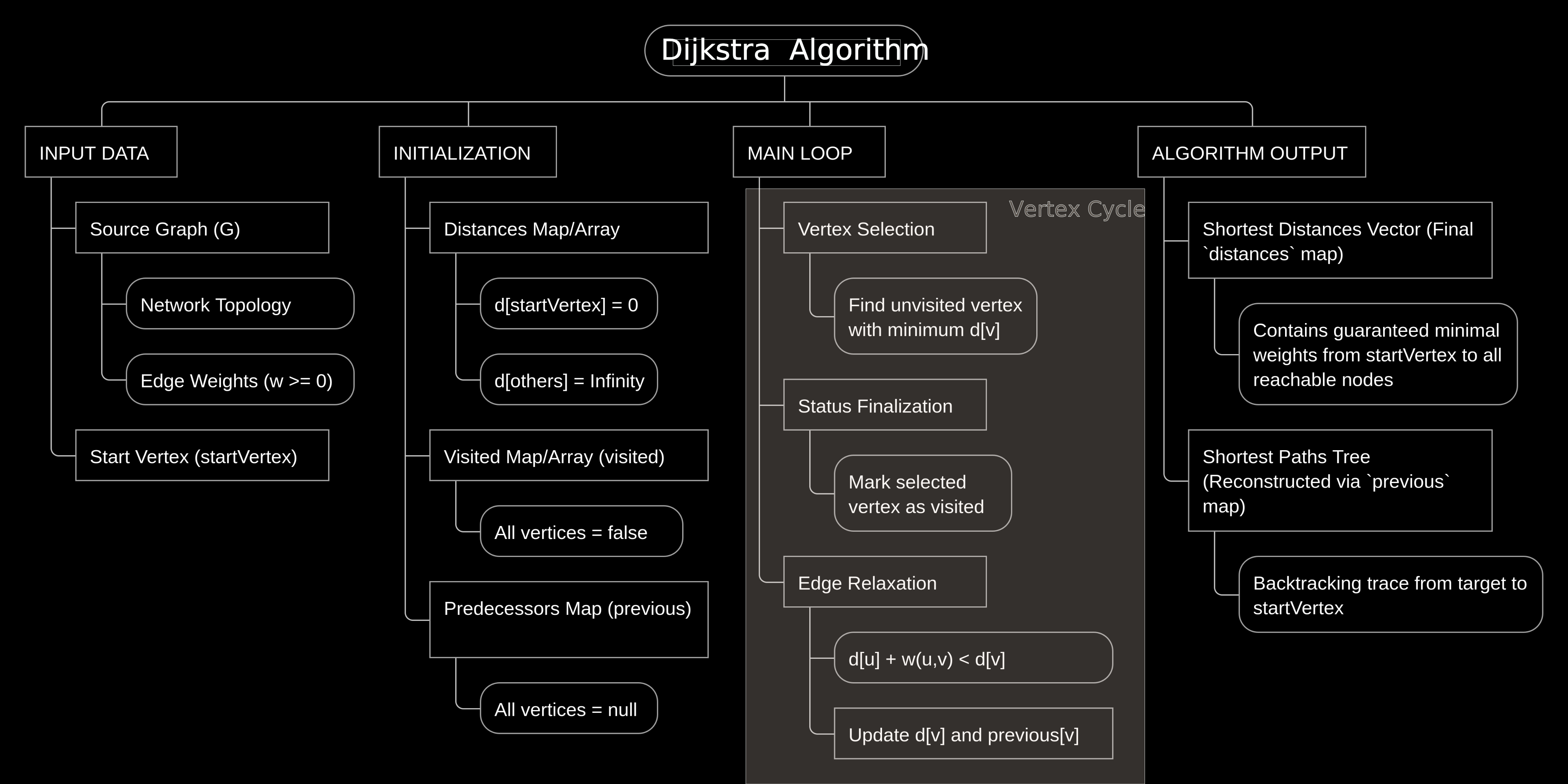
Figure 9.17. Mind map for Dijkstra’s algorithm

Let us examine the algorithm step by step. We start from vertex 0 and find the shortest paths from this vertex to all other vertices of the graph.

To track its progress, the algorithm maintains three essential data structures:

Distance array (distances or d): for each vertex v, distances[v] stores the current length of the shortest known path from the start vertex s to v. Initially, distances[s] = 0, and distances[v] = Infinity for all other vertices.
Visited array (visited): a marker structure where visited[v] = true means that the shortest distance to vertex v has already been finalized. If visited[v] = false, the vertex is still unprocessed.
Previous array (previous): for each vertex v, previous[v] stores the predecessor of v in the currently known shortest path. This structure is used later to reconstruct the actual shortest paths.

The algorithm can be understood through a city-exploration analogy. Imagine a network of cities connected by roads of different lengths. You start at your home city and repeatedly choose the closest city whose shortest route has not yet been finalized. From that city, you check whether its roads provide shorter routes to neighboring cities.

In the classic implementation shown here, the algorithm uses a linear search to find the unvisited vertex with the smallest current distance. This makes the implementation simple and clear for educational purposes.

The functions used in this implementation are summarized in the following table.

Table 3. Functions used in the classic implementation of Dijkstra’s algorithm
Function	Arguments	Purpose	Content	Illustration
`dijkstra`	`graph`, `startVertex`	Main function of the algorithm.	Initializes auxiliary data structures, repeatedly selects the unvisited vertex with the smallest known distance, relaxes outgoing edges, and returns the final shortest distances and predecessors.	`Fig9_17b_dD_dijkstra.svg`
`getVerticesList`	`graph`	Builds the list of graph vertices.	Extracts all vertex names or indices from the graph representation and returns them as a list.	`Fig9_18_getVerticesList.svg`
`initializeDistances`	`vertices`, `startVertex`	Initializes the distance array.	Sets the distance from the start vertex to itself as `0`. Sets the distance to all other vertices as `Infinity`.	`Fig9_19_initData.svg`
`initializeVisited`	`vertices`	Initializes the visited marker array.	Marks all vertices as unvisited. For each vertex `v`, sets `visited[v] = false`.	`Fig9_19_initData.svg`
`initializePrevious`	`vertices`	Initializes the predecessor array.	Sets the predecessor of each vertex to `null`. This structure is later used to reconstruct shortest paths.	`Fig9_19_initData.svg`
`findMinDistanceVertex`	`distances`, `visited`	Finds the next vertex to process.	Searches among all unvisited vertices and returns the vertex with the smallest current distance. If no reachable unvisited vertex exists, returns `null`.	`Fig9_20_findMinDistanceVertex.svg`
`markVertexVisited`	`visited`, `vertex`	Marks the selected vertex as processed.	Sets `visited[vertex] = true`, meaning that the shortest distance to this vertex has been finalized.	`Fig9_21_markVertexVisited.svg`
`relaxEdges`	`graph`, `currentVertex`, `distances`, `previous`, `visited`	Updates distance estimates for neighboring vertices.	For each outgoing edge from `currentVertex` to a neighboring vertex, checks whether the path through `currentVertex` is shorter. If it is shorter, updates `distances[neighbor]` and `previous[neighbor]`.	`Fig9_22_relaxEdges.svg`

DRAKON Diagrams of the Algorithm Functions

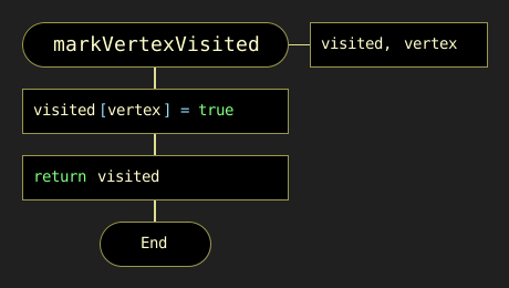
The implementation of Dijkstra’s algorithm is divided into several small functions. Each of them performs one clearly defined operation. This decomposition makes the algorithm easier to understand and easier to verify.

The first helper function builds the list of graph vertices. This list is required to initialize the auxiliary data structures and to iterate over vertices during the search for the next vertex to process.

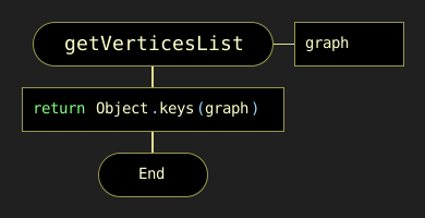
Figure 9.18. Building the list of graph vertices

The next group of functions initializes the main data structures used by the algorithm: the distance array, the visited array, and the predecessor array.

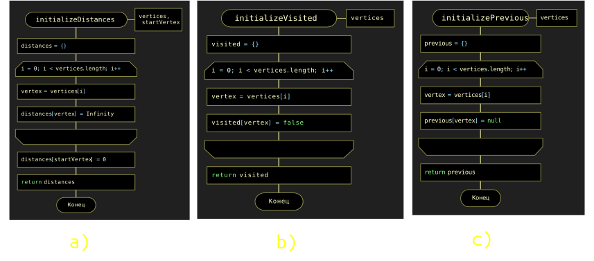
Figure 9.19. Initialization of distance, visited, and predecessor arrays

After initialization, the algorithm must repeatedly choose the unvisited vertex with the smallest currently known distance. This operation is performed by the findMinDistanceVertex function.

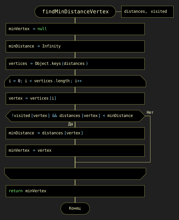
Figure 9.20. Finding the unvisited vertex with the minimum distance

If such a vertex is found, it becomes the current vertex. The algorithm then marks it as processed. This means that the shortest distance to this vertex is now considered final.

Figure 9.21. Marking the selected vertex as processed

The most important operation in the algorithm is edge relaxation. During this step, the algorithm checks whether a shorter path to each neighboring vertex can be obtained through the current vertex.

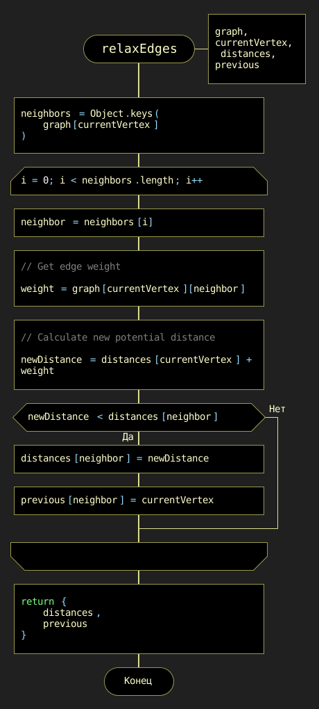
Figure 9.22. Updating distance estimates for neighboring vertices

For an edge from vertex u to vertex v with weight w(u, v), the relaxation condition is:

distances[u] + w(u, v) < distances[v]

If this condition is true, the algorithm updates the current distance estimate:

distances[v] = distances[u] + w(u, v)

and records the predecessor of vertex v:

previous[v] = u

Thus, relaxation performs two tasks at once:

improves the shortest known distance to a vertex;
stores information needed to reconstruct the shortest path.

General Control Flow

The overall logic of the algorithm can be described as follows:

Build the list of graph vertices.
Initialize the distances, visited, and previous structures.
Set the distance to the start vertex to 0.
Find the unvisited vertex with the smallest current distance.
Mark this vertex as visited.
Relax all outgoing edges from this vertex.
Repeat the process until there is no reachable unvisited vertex left.
Return the final distances and previous structures.

A JavaScript implementation of the main function can be written as follows:

function dijkstra(graph, startVertex) {
    const vertices = getVerticesList(graph);

    const distances = initializeDistances(vertices, startVertex);
    const visited = initializeVisited(vertices);
    const previous = initializePrevious(vertices);

    let currentVertex = findMinDistanceVertex(distances, visited);

    while (currentVertex !== null) {
        markVertexVisited(visited, currentVertex);
        relaxEdges(graph, currentVertex, distances, previous, visited);

        currentVertex = findMinDistanceVertex(distances, visited);
    }

    return {
        distances: distances,
        previous: previous
    };
}

The returned object contains two results:

distances — the lengths of the shortest paths from the start vertex to all reachable vertices;
previous — predecessor information that allows the actual shortest paths to be reconstructed.

Result for the Example Graph

Let us run the algorithm from vertex 0. Initially, the distance to vertex 0 is equal to 0, while the distances to all other vertices are set to Infinity.

distances[0] = 0
distances[1] = Infinity
distances[2] = Infinity
distances[3] = Infinity
distances[4] = Infinity
distances[5] = Infinity

After the algorithm finishes, the shortest distances from vertex 0 are:

Table 4. Shortest distances from vertex 0
Vertex	Shortest distance from vertex `0`	Previous vertex
`0`	`0`	`null`
`1`	`48.3`	`0`
`2`	`40.7`	`0`
`3`	`75.6`	`2`
`4`	`60.3`	`5`
`5`	`25.4`	`0`

For example, the shortest path from vertex 0 to vertex 4 is reconstructed using the previous structure:

4 <- 5 <- 0

Reading this sequence in reverse order gives the path:

0 -> 5 -> 4

The total length of this path is:

25.4 + 34.9 = 60.3

Similarly, the shortest path from vertex 0 to vertex 3 is:

0 -> 2 -> 3

with total length:

40.7 + 34.9 = 75.6

Complexity

In this classic implementation, the function findMinDistanceVertex performs a linear scan over all vertices. Since it can be called up to V times, where V is the number of vertices, the vertex-selection part has complexity:

O(V^2)

The relaxation of edges contributes:

O(E)

where E is the number of edges.

Therefore, the total time complexity of this classic implementation is:

O(V^2 + E)

For dense graphs, this is often written simply as:

O(V^2)

More advanced implementations use a priority queue or a min-heap to select the next vertex more efficiently, but the classic version shown here is easier to understand and is well suited for explaining the main idea of Dijkstra’s algorithm.

Computational Experiments with Graph Algorithms

The Graph Constructor provides an interactive environment for investigating graph algorithms.

Students can create directed or undirected graphs, define edge weights, and execute BFS, DFS, and Dijkstra’s shortest-path algorithm.

Run experiment

Section 9. Graphs and Graph Algorithms

9.1. General Information. Basic Terminology

Directed and Undirected Graphs

Undirected Graphs

Directed Graphs

Adjacency, Incidence, and Degree

9.2. Graph Representation Methods

Adjacency Matrix

Adjacency List

Comparison and Complexity

Weighted Graphs

Graph Representation in JavaScript

9.3. Fundamentals of Graph Traversal

Depth-First Search (DFS) — Using Stack (LIFO)

Breadth-First Search (BFS) — Using Queue (FIFO)

Comparison: Stack vs. Queue

DRAKON-Diagrams for DFS and BFS

Choosing Between DFS and BFS

9.4. Calculation of Paths and Travel Costs Between Two Vertices

General Idea of the Algorithm

Functional Structure of the Path Search Module

Description of Key Functions

initPathSearch(graph, source, target)

findPathWithContext(current, context)

handleFoundPath(context)

prepareMoveToNeighbor(context, current, neighbor)

Reversing function backtrackFromNeighbor(context, neighbor, oldState)

Algorithmic Complexity Analysis

Program Execution Example

Summary

9.5. Dijkstra’s Algorithm

Graph Representation for Dijkstra’s Algorithm

How the Algorithm Works

DRAKON Diagrams of the Algorithm Functions

General Control Flow

Result for the Example Graph

Complexity

Computational Experiments with Graph Algorithms

Reversing function `backtrackFromNeighbor(context, neighbor, oldState)`