Section 7. Basic Sorting Algorithms
This section provides a comprehensive analysis of fundamental sorting algorithms for contiguous memory segments (array slices). It explores core concepts, algorithmic mechanics, and performance trade-offs across classic comparison-based methods: Bubble Sort, Selection Sort, Insertion Sort, Quick Sort, Merge Sort, Shell Sort, and Heap Sort. Each algorithm is evaluated in terms of best, average, and worst-case time complexity, auxiliary space requirements, and numerical stability. To enhance pedagogical clarity and structural logic, visual workflow formalisms—including DRAKON diagrams, step-by-step state transition tables, and heap tree visualizations—are systematically integrated. Finally, a comparative framework is established to guide optimal algorithm selection based on key data characteristics and constraints.
7.1. General Characteristics of Sorting Algorithms
Sorting is one of the most common operations in data processing — not only in computer science, but in many areas of human activity. In computing, sorting algorithms are used everywhere: in databases, search engines, operating systems, and beyond.
At its core, the goal of sorting is simple: given a list of records (each with a key value), we want to reorder the list so that the keys are arranged in increasing or decreasing order. This makes it easier to work with the data — especially when we need to search or analyze it later.
Over time, many sorting algorithms have been developed. Some are easy to implement and work well for small datasets, but become inefficient as the dataset grows. Others are designed for large collections and offer better performance, though they may be more complex to understand or implement.
To help understand how these algorithms work, especially the more complex ones, we will use visual explanations. In this book, we include DRAKON-diagrams and illustrations to make the logic clear and accessible.
Since most sorting tasks in programming involve arrays or similar structures, this section focuses on sorting slices (contiguous segments of arrays).
7.2. Bubble Sort
Bubble Sort is one of the simplest sorting algorithms, especially suitable for small datasets. The algorithm gets its name from the way larger values "bubble up" to the end of the array with each pass. The DRAKON-diagram of the algorithm is shown in Figure 7.1.
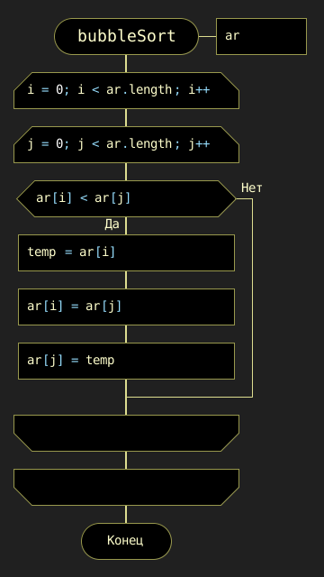
The algorithm uses two nested loops. For each index i, it iterates over the remaining elements with index j. At each step, the values arr[i] and arr[j] are compared. If arr[j] is smaller than arr[i], the two elements are swapped. This process pushes the largest unsorted value toward the end of the array during each outer loop iteration.
The following table shows the results of sorting a series of values for each outer loop parameter (i).
| j=0 | j=1 | j=2 | j=3 | j=4 | j=5 | j=6 | j=7 | j=8 | j=9 |
|---|---|---|---|---|---|---|---|---|---|
90 |
11 |
81 |
21 |
71 |
31 |
61 |
41 |
51 |
10 |
11 |
90 |
81 |
21 |
71 |
31 |
61 |
41 |
51 |
10 |
11 |
81 |
90 |
21 |
71 |
31 |
61 |
41 |
51 |
10 |
11 |
21 |
81 |
90 |
71 |
31 |
61 |
41 |
51 |
10 |
11 |
21 |
71 |
81 |
90 |
31 |
61 |
41 |
51 |
10 |
11 |
21 |
31 |
71 |
81 |
90 |
61 |
41 |
51 |
10 |
11 |
21 |
31 |
61 |
71 |
81 |
90 |
41 |
51 |
10 |
11 |
21 |
31 |
51 |
61 |
71 |
81 |
90 |
51 |
10 |
11 |
21 |
31 |
41 |
51 |
61 |
71 |
81 |
90 |
10 |
10 |
11 |
21 |
31 |
41 |
51 |
61 |
71 |
81 |
90 |
The time complexity of Bubble Sort is quite high — O(n²). This is due to the large number of comparisons (arr[j] < arr[i]) and possible swaps. However, the space complexity is O(1), since no additional memory is needed beyond the original array.
The algorithm is stable, meaning that equal elements retain their original order after sorting.
Because of its simplicity, Bubble Sort is still used in some applications — for example, in computer graphics. There, it is helpful for correcting small errors in nearly sorted arrays, often completing in linear time (about 2n steps). However, it is highly inefficient for large datasets.
7.3. Selection Sort
The Selection Sort algorithm is based on comparison operations. It works by dividing the dataset into two parts: the sorted portion on the left and the unsorted portion on the right. The DRAKON-diagram of this algorithm is shown in Figure 7.2.
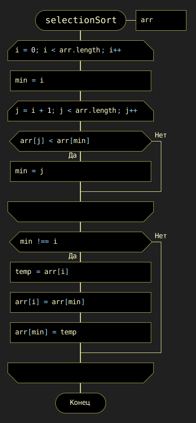
The idea is simple: in each iteration, the algorithm finds the smallest value in the unsorted part and swaps it with the first unsorted element. Initially, the sorted part is empty, and the unsorted part is the entire array.
For example, given the set [90, 12, 83, 24, 75, 38, 62, 41, 59, 10], the algorithm scans the array and finds the smallest element — 10. It then swaps 10 with the element at the first position (90). The sorted part now contains 10, and the process repeats with the remaining elements. The table below illustrates this process of selection and replacement.
90 |
12 |
83 |
24 |
75 |
38 |
62 |
41 |
59 |
10 |
10 |
12 |
83 |
24 |
75 |
38 |
62 |
41 |
59 |
90 |
10 |
12 |
83 |
24 |
75 |
38 |
62 |
41 |
59 |
90 |
10 |
12 |
83 |
24 |
75 |
38 |
62 |
41 |
59 |
90 |
10 |
12 |
24 |
83 |
75 |
38 |
62 |
41 |
59 |
90 |
10 |
12 |
24 |
38 |
75 |
83 |
62 |
41 |
59 |
90 |
10 |
12 |
24 |
38 |
41 |
83 |
62 |
75 |
59 |
90 |
10 |
12 |
24 |
38 |
41 |
59 |
62 |
75 |
83 |
90 |
10 |
12 |
24 |
38 |
41 |
59 |
62 |
75 |
83 |
90 |
10 |
12 |
24 |
38 |
41 |
59 |
62 |
75 |
83 |
90 |
Note to the table: Underlined items are already sorted; selected items are minimal in the current pass.
The time and space complexity of the Selection Sort algorithm are summarized in the table below:
| Time Complexity | |
|---|---|
Worst case |
O(n²) |
Average case |
O(n²) |
Best case |
O(n²) |
Space Complexity |
|
All cases |
O(1) |
The time complexity is the same in all cases because the algorithm uses two nested loops:
-
The outer loop runs n times (once per element)
-
The inner loop runs (n - 1) times per outer iteration
-
This results in a total of n * (n - 1) comparisons, which gives the time complexity of O(n²) regardless of the input order.
7.4. Insertion Sort
Insertion Sort works by repeatedly taking an item from the unsorted part of the array and inserting it into its correct position in the sorted part. This process continues until all items are sorted.
This algorithm is similar to how people naturally sort playing cards or paper documents: taking one item at a time and inserting it into the correct place. The DRAKON-diagram for the Insertion Sort algorithm is shown in Figure 7.3.
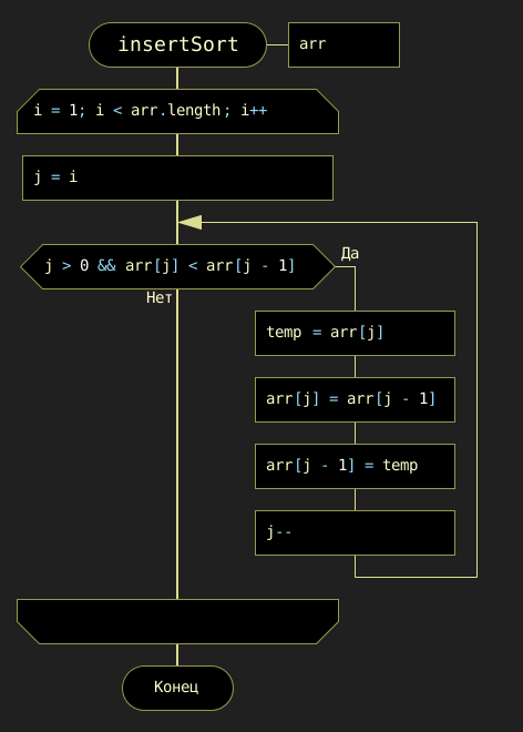
In this algorithm, larger values are pushed to the right. The algorithm compares adjacent elements and swaps them if needed. This process is shown in the table below, where underscores mark the positions where swaps occurred.
Input array |
|||||||||
90 |
11 |
81 |
21 |
71 |
31 |
61 |
41 |
51 |
10 |
i = 1 |
|||||||||
11 |
90 |
81 |
21 |
71 |
31 |
61 |
41 |
51 |
10 |
i = 2 |
|||||||||
11 |
81 |
90 |
21 |
71 |
31 |
61 |
41 |
51 |
10 |
i = 3 |
|||||||||
11 |
81 |
21 |
90 |
71 |
31 |
61 |
41 |
51 |
10 |
11 |
21 |
81 |
90 |
71 |
31 |
61 |
41 |
51 |
10 |
i = 4 |
|||||||||
11 |
21 |
81 |
71 |
90 |
31 |
61 |
41 |
51 |
10 |
11 |
21 |
71 |
81 |
90 |
31 |
61 |
41 |
51 |
10 |
i = 5 |
|||||||||
11 |
21 |
71 |
81 |
31 |
90 |
61 |
41 |
51 |
10 |
11 |
21 |
71 |
31 |
81 |
90 |
61 |
41 |
51 |
10 |
11 |
21 |
31 |
71 |
81 |
90 |
61 |
41 |
51 |
10 |
i = 6 |
|||||||||
11 |
21 |
31 |
71 |
81 |
61 |
90 |
41 |
51 |
10 |
11 |
21 |
31 |
71 |
61 |
81 |
90 |
41 |
51 |
10 |
11 |
21 |
31 |
61 |
71 |
81 |
90 |
41 |
51 |
10 |
i = 7 |
|||||||||
11 |
21 |
31 |
61 |
71 |
81 |
41 |
90 |
51 |
10 |
11 |
21 |
31 |
61 |
71 |
81 |
41 |
51 |
90 |
10 |
11 |
21 |
31 |
61 |
41 |
71 |
81 |
90 |
51 |
10 |
11 |
21 |
31 |
41 |
61 |
71 |
81 |
90 |
51 |
10 |
i = 8 |
|||||||||
11 |
21 |
31 |
41 |
61 |
71 |
81 |
51 |
90 |
10 |
11 |
21 |
31 |
41 |
61 |
71 |
51 |
81 |
90 |
10 |
11 |
21 |
31 |
41 |
61 |
51 |
71 |
81 |
90 |
10 |
11 |
21 |
31 |
41 |
51 |
61 |
71 |
81 |
90 |
10 |
i = 9 |
|||||||||
11 |
21 |
31 |
41 |
51 |
61 |
71 |
81 |
10 |
90 |
11 |
21 |
31 |
41 |
61 |
51 |
71 |
10 |
81 |
90 |
11 |
21 |
31 |
41 |
51 |
61 |
71 |
10 |
81 |
90 |
11 |
21 |
31 |
41 |
51 |
61 |
10 |
71 |
81 |
90 |
11 |
21 |
31 |
41 |
51 |
10 |
61 |
71 |
81 |
90 |
11 |
21 |
31 |
41 |
10 |
51 |
61 |
71 |
81 |
90 |
11 |
21 |
31 |
10 |
41 |
51 |
61 |
71 |
81 |
90 |
11 |
21 |
10 |
31 |
41 |
51 |
61 |
71 |
81 |
90 |
11 |
10 |
21 |
31 |
41 |
51 |
61 |
71 |
81 |
90 |
10 |
11 |
21 |
31 |
41 |
51 |
61 |
71 |
81 |
90 |
The time complexity of Insertion Sort depends on how the elements are arranged in the input array:
- Worst case
-
when the array is sorted in reverse order. Each element must be compared with all previous elements and moved to the beginning of the array. The number of operations is n(n - 1) / 2 → O(n²).
- Average case
-
when the array is partially sorted. Each element is compared, on average, with half of the previous elements: (n²) / 4 → O(n²).
- Best case
-
when the array is already sorted. Each element is compared with only the one before it: (n - 1) → O(n).
The complexity summary is given in the table below:
| Time Complexity | |
|---|---|
Worst case |
O(n²) |
Average case |
O(n²) |
Best case |
O(n) |
Space complexity |
O(1) |
7.5. Quick Sort
Quick Sort is a highly efficient sorting algorithm based on the divide-and-conquer strategy. Its general scheme includes the following steps:
-
Select a pivot (reference) element from the array slice.
-
Partition the array so that all elements smaller than the pivot are placed before it, and all greater or equal — after it.
-
Recursively apply this procedure to the left and right partitions.
-
As a result, the array becomes fully sorted.
The DRAKON-diagram of the Quick Sort algorithm is shown in Figure 7.4.
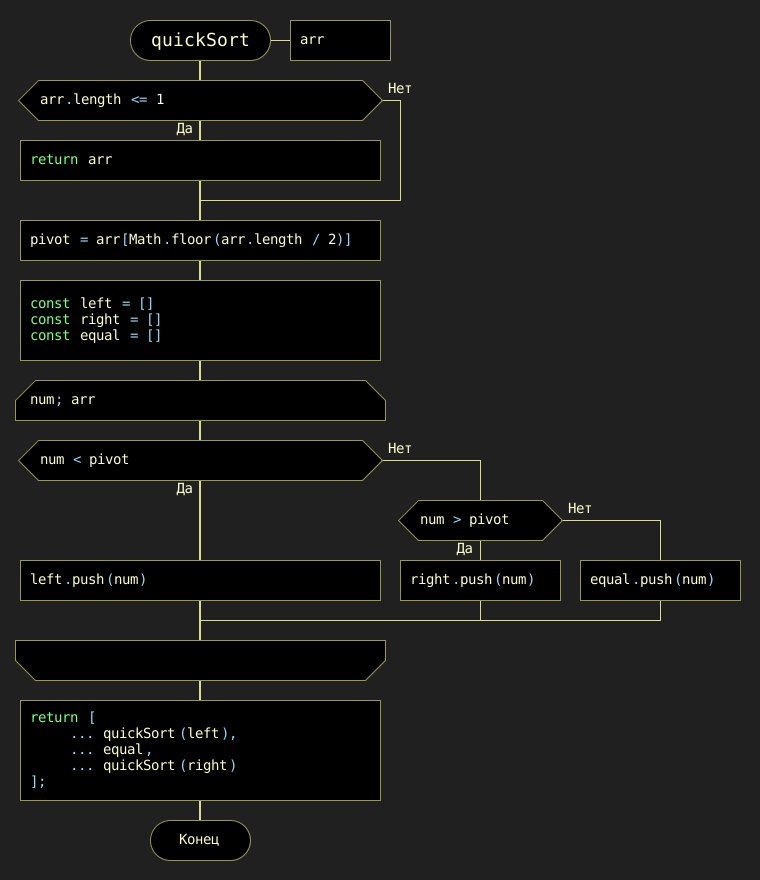
Let us look at an example in detail. Suppose we are sorting the array [78, 11, 81, 21, 71, 31, 61, 41, 51, 24], and we choose 31 as the pivot.
78 |
11 |
81 |
21 |
71 |
31 |
61 |
41 |
51 |
24 |
We create three temporary arrays:
-
left[] for elements less than the pivot
-
equal[] for elements equal to the pivot
-
right[] for elements greater than the pivot
During execution, if an element from the left side is greater than the pivot, and one from the right side is smaller, the two elements are swapped. In our example, 78 > 31 and 24 < 31, so they are exchanged. This process continues until the subarray is partitioned correctly. Then, Quick Sort is applied recursively to the left and right partitions.
To better understand how recursive sorting builds the final result, the table below shows how the quickSort function combines the left, equal, and right parts at each step:
| Step | Left | Pivot | Right | Result = left + equal + right |
|---|---|---|---|---|
[78, 11, 81, 21, 71, 31, 61, 41, 51, 24] |
11, 21, 24 |
31 |
78, 81, 71, 61, 41, 51 |
– |
[11, 21, 24] |
11 |
21 |
24 |
11, 21, 24 |
[78, 81, 71, 61, 41, 51] |
41, 51 |
61 |
78, 81, 71 |
11, 21, 24 |
[41, 51] |
41 |
51 |
11, 21, 24, 41, 51 |
|
[78, 81, 71] |
78, 71 |
81 |
11, 21, 24, 41, 51, 61 |
|
[78, 71] |
71 |
78 |
11, 21, 24, 41, 51, 61, 71, 78 |
|
[81] |
81 |
11, 21, 24, 41, 51, 61, 71, 78, 81 |
The time complexity of Quick Sort depends on how well the pivot is chosen:
-
Best case: the pivot is the median → O(n log n)
-
Average case: still O(n log n), due to recursive halving
-
Worst case: when the pivot is the smallest or largest item, resulting in unbalanced partitions → O(n²)
Quick Sort uses recursion. In each step, it partitions the array and performs O(n) work. This leads to the recurrence relation T(n) = 2T(n/2) + O(n), which solves to O(n log n).
The complexity summary is shown below. Quick Sort is not stable by default.
| Time Complexity | |
|---|---|
Worst case |
O(n²) |
Average case |
O(n log n) |
Best case |
O(n log n) |
Space Complexity |
|
Worst case |
O(n) |
Average case |
O(log n) |
7.6. Merge Sort
Merge Sort is a classic divide-and-conquer algorithm. It works by recursively splitting the array into smaller parts until each part contains only one element (trivially sorted). After the splitting phase, the algorithm merges the sorted parts back together.
During merging, one element from each fragment is selected and compared. The smaller (or larger, depending on the desired order) element is added to the result array. The process continues until all elements are merged. Figure 7.5 illustrates this process:
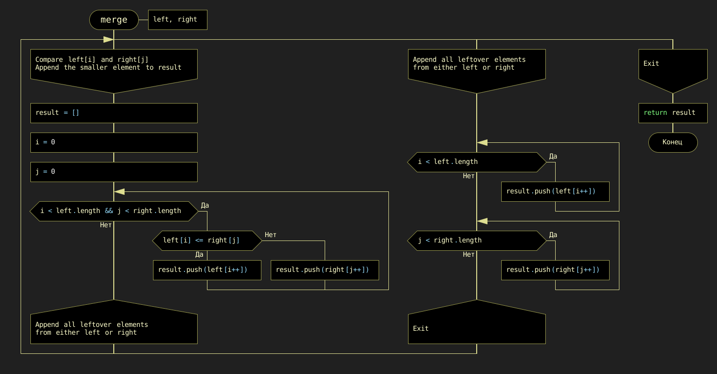
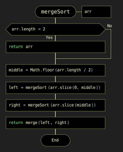
Figure 7.5. DRAKON-diagrams of Merge Sort algorithm: a) merge() function; b) mergeSort() function
A visual representation of splitting and merger phases are shown in Figure 7.6.
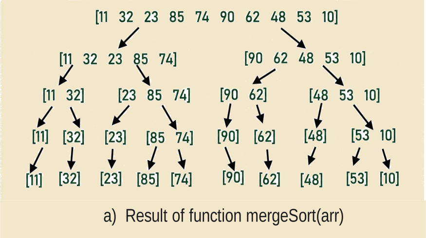
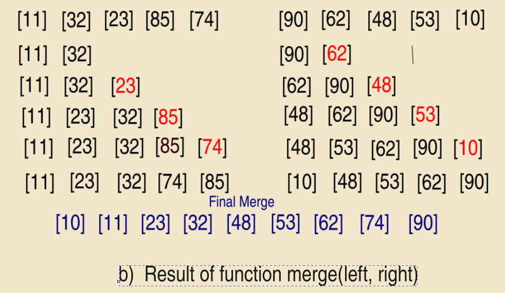
Figure 7.6. Visual representation of Merge Sort algorithm: a) splitting phase; b) merging phase
Merge Sort has a time complexity of O(n log n), where n is the number of elements in the array. The algorithm splits the array into two halves until only single elements remain. The number of split operations is O(log n), and each merge operation compares n elements, which gives the overall complexity of O(n log n).
The summary of time and space complexity is shown below:
| Time Complexity | |
|---|---|
Worst case |
O(n log n) |
Average case |
O(n log n) |
Best case |
O(n log n) |
Space Complexity |
|
Worst case |
O(n) |
Average case |
O(n) |
Best case |
O(n) |
Merge Sort is a stable sorting algorithm, which means it preserves the relative order of equal elements in the input array. This stability is achieved because, during the merge phase, if two elements are equal, the one from the left subarray is placed before the one from the right subarray.
7.7. Shell Sort
Shell Sort is a variation of Insertion Sort. It begins by comparing and sorting elements that are separated by a certain distance d. Then, the process is repeated for smaller values of d until d = 1, which is equivalent to a standard insertion sort.
The DRAKON-diagram of the Shell Sort algorithm is shown in Figure 7.7.
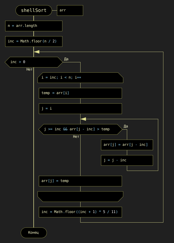
Figure 7.7. DRAKON-diagram of the Shell Sort algorithm
Shell Sort uses a three-step process common to many sorting algorithms:
-
Segmenting the array
-
Sorting within the segments
-
Merging the results into a sorted array
The array is partitioned in such a way that each item in a segment is a fixed number of positions apart from the others. This introduces a challenge: choosing the best distance d. A simple example of such a sequence is: d = n / 2, then d = d / 2, and so on, until d = 1.
The table illustrates how elements are swapped when a smaller value is found at position arr[j] compared to arr[j - inc].
inc = 5
j |
0 |
1 |
2 |
3 |
4 |
5 |
6 |
7 |
8 |
9 |
90 |
-80 |
70 |
-60 |
50 |
-40 |
30 |
-20 |
10 |
0 |
|
-40 |
-80 |
-20 |
-60 |
50 |
90 |
30 |
70 |
10 |
0 |
|
-40 |
-80 |
-20 |
-60 |
0 |
90 |
30 |
70 |
10 |
50 |
inc = 2
j |
0 |
1 |
2 |
3 |
4 |
5 |
6 |
7 |
8 |
9 |
-40 |
-80 |
-20 |
-60 |
0 |
70 |
30 |
90 |
10 |
50 |
|
-40 |
-80 |
-20 |
-60 |
0 |
70 |
10 |
90 |
30 |
50 |
|
-40 |
-80 |
-20 |
-60 |
0 |
70 |
10 |
90 |
30 |
50 |
|
-40 |
-80 |
-20 |
-60 |
0 |
50 |
10 |
70 |
30 |
90 |
inc = 1
j |
0 |
1 |
2 |
3 |
4 |
5 |
6 |
7 |
8 |
9 |
-40 |
-80 |
-20 |
-60 |
0 |
50 |
10 |
70 |
30 |
90 |
|
-80 |
-40 |
-60 |
-20 |
0 |
50 |
10 |
70 |
30 |
90 |
|
-80 |
-60 |
-40 |
-20 |
0 |
50 |
10 |
70 |
30 |
90 |
|
-80 |
-60 |
-40 |
-20 |
0 |
10 |
50 |
70 |
30 |
90 |
|
-80 |
-60 |
-40 |
-20 |
0 |
10 |
50 |
30 |
70 |
90 |
|
-80 |
-60 |
-40 |
-20 |
0 |
10 |
30 |
50 |
70 |
90 |
The average time complexity of Shell Sort is estimated as O(n · log² n), though this depends on multiple factors.
First, Shell Sort is essentially a generalization of Insertion Sort that uses gap-based comparisons. Second, the performance depends on the choice of gap sequence — that is, the values of d used during sorting. Different sequences can yield significantly different results.
Because Shell Sort works by refining the array through a series of passes with decreasing gaps, its time complexity is sensitive to these gap values. The optimal gap sequence is still a subject of research, and no single sequence is universally optimal.
As a result, although the average-case complexity is commonly cited as O(n · log² n), the exact performance may vary depending on the input and the sequence used.
Shell Sort is not stable in its original form, but it can be modified to preserve stability if needed.
7.8. Heap Sort
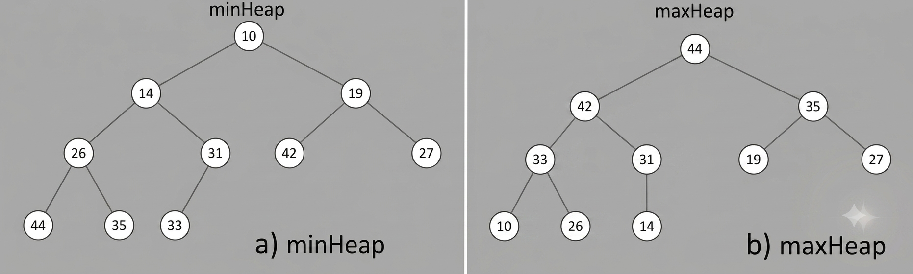
Heap Sort (pyramid sorting) can be seen as an improved version of Selection Sort: it divides the input data into sorted and unsorted regions, and then successively reduces the unsorted region by removing the largest item and moving it to the sorted region. The improvement is that a binary heap is used to find the highest value, not a linear search algorithm.
This algorithm is executed using the notion of a heap, which is a complete binary tree (see subsection 1.3).In a max-heap, parent nodes are greater than or equal to their children, whereas in a min-heap, parent nodes are less than or equal to their children. A binary heap tree can be of two types:
- MinHeap
-
the parent node is always smaller than the child nodes
- MaxHeap
-
the parent node is always greater than or equal to the child nodes
Figure 7.8 shows examples of both:
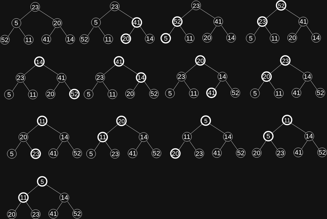
The sequence of heap construction steps is shown in the table below:
| 23 | 5 | 20 | 52 | 11 | 41 | 14 |
|---|---|---|---|---|---|---|
23 |
5 |
41 |
52 |
11 |
20 |
14 |
23 |
52 |
41 |
5 |
11 |
20 |
14 |
52 |
23 |
41 |
5 |
11 |
20 |
14 |
14 |
23 |
41 |
5 |
11 |
20 |
52 |
41 |
23 |
14 |
5 |
11 |
20 |
52 |
20 |
23 |
14 |
5 |
11 |
41 |
52 |
23 |
20 |
14 |
5 |
11 |
41 |
52 |
11 |
20 |
14 |
5 |
23 |
41 |
52 |
20 |
11 |
14 |
5 |
23 |
41 |
52 |
5 |
11 |
14 |
20 |
23 |
41 |
52 |
11 |
5 |
14 |
20 |
23 |
41 |
52 |
5 |
11 |
14 |
20 |
23 |
41 |
52 |
The Heap Sort algorithm uses three functions:
heapSort-
performs the main sorting by rearranging nodes
heapify-
compares adjacent nodes to maintain heap property
swap-
swaps two nodes
The sequence of node movements in the heap is shown in Figure 7.9:
DRAKON-diagrams of the Heap Sort algorithm are presented in Figure 7.10:
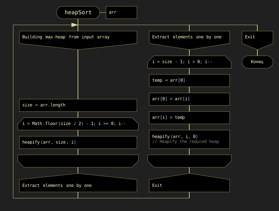
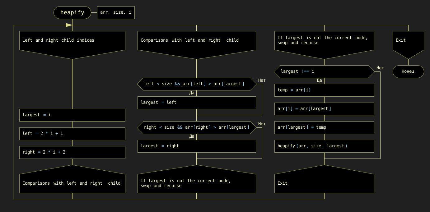
Figure 7.10. DRAKON-diagram of Heap Sort algorithm: a) heapSort(arr); b) heapify(arr, size, i)
The time complexity of Heap Sort is O(n log n) for all cases (worst, average, and best). The space complexity is O(1) as it sorts in place. Heap Sort is not stable.
7.9. Comparison of Sorting Algorithms
Choosing a sorting algorithm is determined by the following factors:
-
Time complexity
-
Space complexity
-
Stability
Knowing the strengths and weaknesses of each of the algorithms considered allows you to make a choice in favor of a particular sort. Each algorithm is unique and works best under certain conditions.
Time Complexity Comparison
| Algorithm | Worst | Average | Best |
|---|---|---|---|
Bubble Sort |
O(n²) |
O(n²) |
O(n) |
Selection Sort |
O(n²) |
O(n²) |
O(n²) |
Insertion Sort |
O(n²) |
O(n²) |
O(n) |
Quick Sort |
O(n²) |
O(n log n) |
O(n log n) |
Merge Sort |
O(n log n) |
O(n log n) |
O(n log n) |
Shell Sort |
O(n·log² n) |
O(n·log² n) |
O(n) |
Heap Sort |
O(n log n) |
O(n log n) |
O(n log n) |
Space Complexity and Stability Comparison
| Algorithm | Space Complexity | Stable |
|---|---|---|
Bubble Sort |
O(1) |
Yes |
Selection Sort |
O(1) |
No |
Insertion Sort |
O(1) |
Yes |
Quick Sort |
O(log n) average, O(n) worst |
No |
Merge Sort |
O(n) |
Yes |
Shell Sort |
O(1) |
No |
Heap Sort |
O(1) |
No |
Some common sorting algorithms are inherently stable, such as Merge Sort, Insertion Sort, and Bubble Sort. Others, such as Quick Sort, Heap Sort, and Selection Sort, are unstable. However, stability can often be achieved in unstable algorithms by using additional space or modifying the implementation.
Computational Experiment
The user enters an array and a target value, or selects "Random sorted array" / "Random unsorted array".
Clicking "Run all searches" executes all three algorithms against the same dataset.
A results table displays the output and the number of comparisons made by each algorithm, followed by a step-by-step trace.
More information about the experiment can be found in the App by activating the "Launch Sorting Experiment" button.