Section 6. Basic Search Algorithms

This section examines the primary algorithms used for searching data structures. To enhance the understanding of the practical applications of these algorithms, DRAKON-diagrams are provided along with assessments of their time and space complexity.

Searching is one of the most important algorithms for processing data structures. Search algorithms are designed to check the presence of an element or extract an element from any data structure in which it is stored. More strictly, the search problem can be formulated as follows: find one or more elements in a set, where the elements sought must have a certain property. This property can be absolute or relative. A relative property characterizes an element with respect to other elements: for example, a minimum element in a set of numbers.

There are many search algorithms. Their complexity varies from simple sequential search algorithms to highly efficient binary search algorithms, which, however, require sorted datasets. Of particular note are algorithms based on presenting the core set of data in a different, more searchable form, which are used in real-world applications for processing data sets in huge databases.

There is no single algorithm to solve all search problems. Some algorithms run faster than others but require additional RAM to run. Others run very quickly but can only be used for pre-sorted arrays. At the same time, the analysis of search algorithms is somewhat different from sorting algorithms. In particular, there is no stability problem for them. However, there may be situations that require the introduction of new criteria of complexity and its assessment. In general, all algorithms are reduced to the following steps:

Establishing the property of the elements of the source set; in most cases, these are the values of the elements.
Matching the value of the element with the reference property (for absolute properties) or comparing the properties of two elements (for relative properties).
Traversing the elements of the set.

Fundamentally, search algorithms are categorized by their underlying search paradigms and strategies. Based on the type of search operation, these algorithms are usually classified into two categories:

Sequential Search: The list or array is traversed sequentially and each element is checked.
Interval Search: These algorithms are specifically designed for searching in sorted data structures. These types of search algorithms are much more efficient than linear search because they repeatedly target the center of the search structure and divide the search space in half.

6.1. Linear Data Searching

a) Linear Search of Unsorted Data

In the case of a linear search for an element in an unordered dataset, for example, in an array or in a slice, the simplest algorithm is to examine all elements until the desired value is found (Figure 6.1).

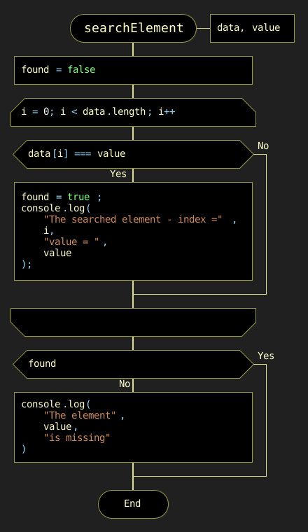
Figure 6.1. DRAKON-diagram of the Linear Search Algorithm

This algorithm is not very efficient, but it works on arbitrary collections. Time complexity: O(n). In the worst case (the desired element is in the last position), to find the element you need to traverse all elements. Here "n" is the size of the slice. Space complexity: O(1). No additional memory is required to accommodate the slice. Another worst-case scenario is the absence of the required element.

b) Linear Search of Sorted Data

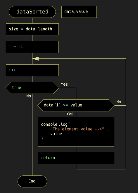
If the elements of the dataset are sorted in ascending or descending order, finding the desired element is much more efficient than in an unordered linear search. In many cases, you do not have to traverse the whole list. For example, when traversing an ascending sorted list, if an element with a higher value than the search key is encountered, the search is stopped. This approach saves time and increases productivity. Figure 6.2 shows the DRAKON-diagram of this algorithm.

Figure 6.2. DRAKON-diagram of the Search in a Sorted Array

6.2. Binary Search for Data in a Sorted Structure

Binary search is performed as follows:

Determine the value of the element in the middle of the data structure. The resulting value is compared to the value being searched for.
If the search value is less than the middle value, the search is carried out in the first half of the elements; otherwise, in the second half.
The search continues by determining the value of the middle element in the selected half and comparing it to the key.
The process continues until an element with the search value is found or the search interval is empty.

The DRAKON-diagram of the binary search algorithm is represented in Figure 6.3 (the main() module is similar to the previous algorithm):

Figure 6.3. DRAKON-diagram of the Binary Search Algorithm

Time complexity of the binary search algorithm belongs to class O(log n). This means that the asymptotic increase in the time taken by the function to process an input set of size n will not exceed log n. Space complexity: O(1) for the iterative implementation.

6.3. Searching and Related Operations in a Singly Linked List

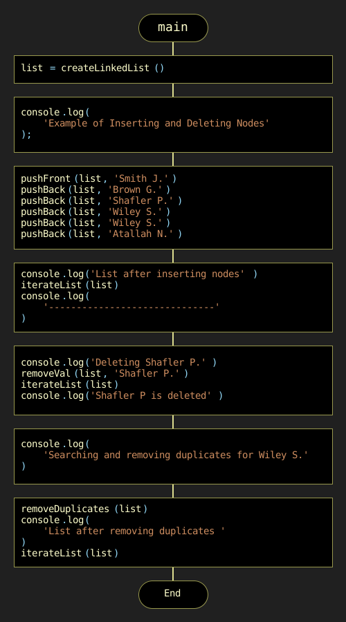
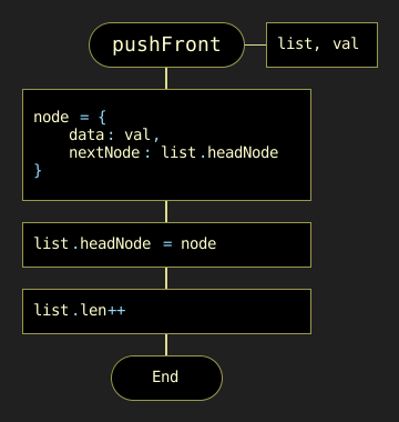
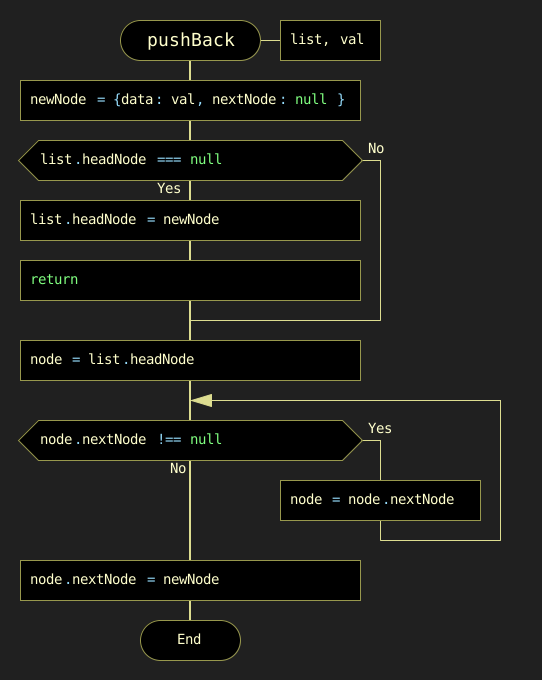
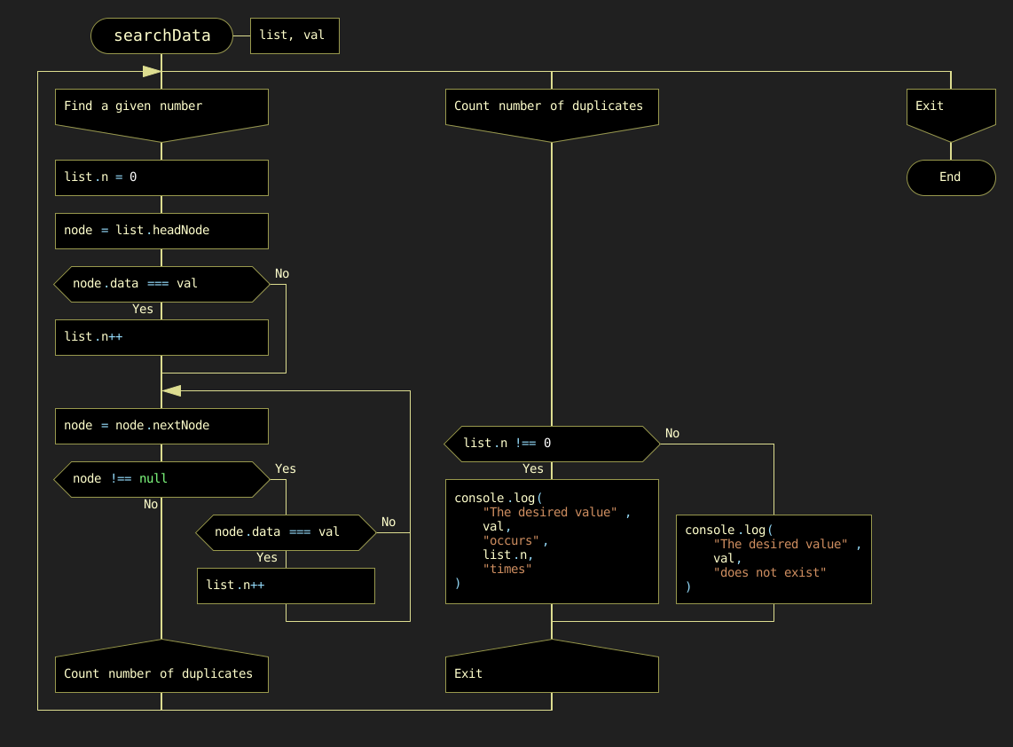
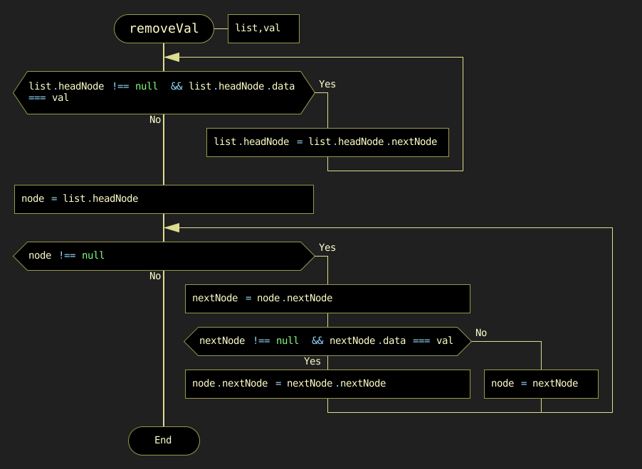
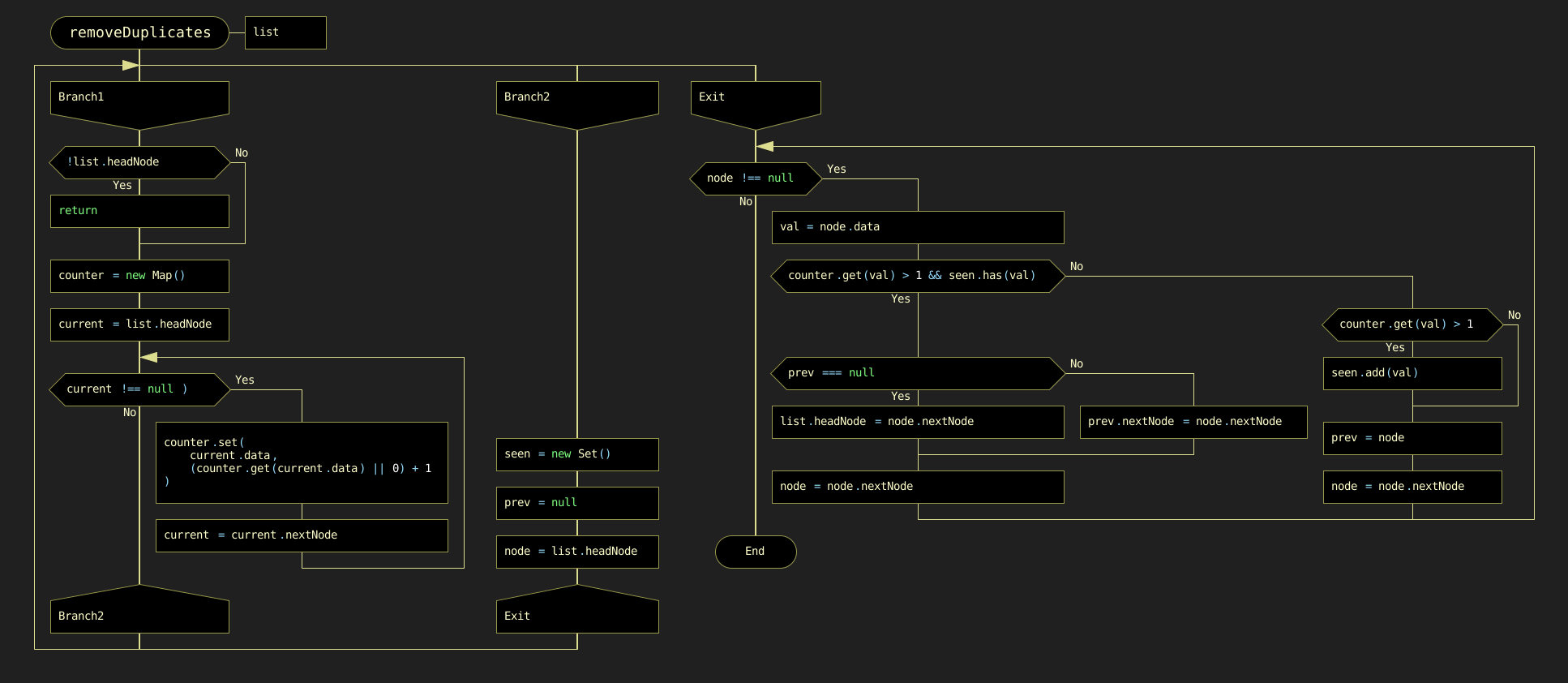
There are three possibilities for a singly linked list. First, the desired value is missing from the list. Second, the desired value appears once. Third, the desired value appears multiple times. You can also set the task of removing duplicates — nodes that are redundant. To solve these problems, it is necessary to create a singly linked list whose items contain values "Smith J.", "Brown G.", "Shafler P.", "Wiley S.", "Wiley S.", "Atallah N.". In this list you should delete the entry "Brown G." and then add a new entry "Singer B." placing it after the entry "Wiley S.". After that, you should delete duplicates of the entry "Wiley S." leaving only one. The linked list operations below demonstrate search as a subroutine in deletion, insertion and duplicate removal — all of which rely on locating an element by value. The corresponding DRAKON-diagrams are presented in Figure 6.4.

a) Function main() as the Entry Point for Linked List Operations

b) Functions for Pushing New Items (pushFront(list, val)

c) Functions for Pushing New Items pushBack(list, val))

d) Function for Searching (searchData(val))

e) Function for Deletion (removeVal(val))

f) Function for Removing Duplicates (removeDuplicates)

Execution Results

Figure 6.4. DRAKON-diagrams of linked list algorithms: deletion, search and duplicate deletion

Results of the execution of the above algorithms are as follows:

List after inserting nodes:
Smith J.
Brown G.
Shafler P.
Wiley S.
Wiley S.
Atallah N.

Deleting `Shafler P.`
`Shafler P.` is deleted
List after inserting nodes
Smith J.
Brown G.
Shafler P.
Wiley S.
Wiley S.
Atallah N.

Deleting `Shafler P.`
`Shafler P.` is deleted
List after deletion
Smith J.
Brown G.
Wiley S.
Wiley S.
Atallah N.

Searching and removing duplicates for `Wiley S.`
The desired value Wiley S. occurs 2 times
List after removing duplicates
Smith J.
Brown G.
Wiley S.
Atallah N.

List after inserting nodes
Smith J.
Brown G.
Shafler P.
Wiley S.
Wiley S.
Atallah N.

Deleting `Shafler P.`
Shafler P. is deleted
List after deletion
Smith J.
Brown G.
Wiley S.
Wiley S.
Atallah N.

Searching and removing duplicates for `Wiley S.`
The desired value Wiley S. occurs 2 times
List after removing duplicates
Smith J.
Brown G.
Wiley S.
Atallah N.

6.4. Hashing

The time to find an item in a data set often depends on how many comparisons are made. To improve search efficiency, the number of key comparisons must be minimized. One way is to map keys to a smaller range of indices – this process is called hashing, and the resulting structure is a hash table.

In terms of abstract data type (ADT) theory, a hash table implements an associative array. It stores key‑value pairs and supports three basic operations: insert (add a pair), lookup (find a value by key), and delete (remove a pair).

From a programming perspective, a hash table consists of buckets — groups of elements mapped to the same hash index. The hash function transforms a given key into an integer index (the bucket number). Many methods exist to construct a hash function, some of which are shown in Figure 6.5.

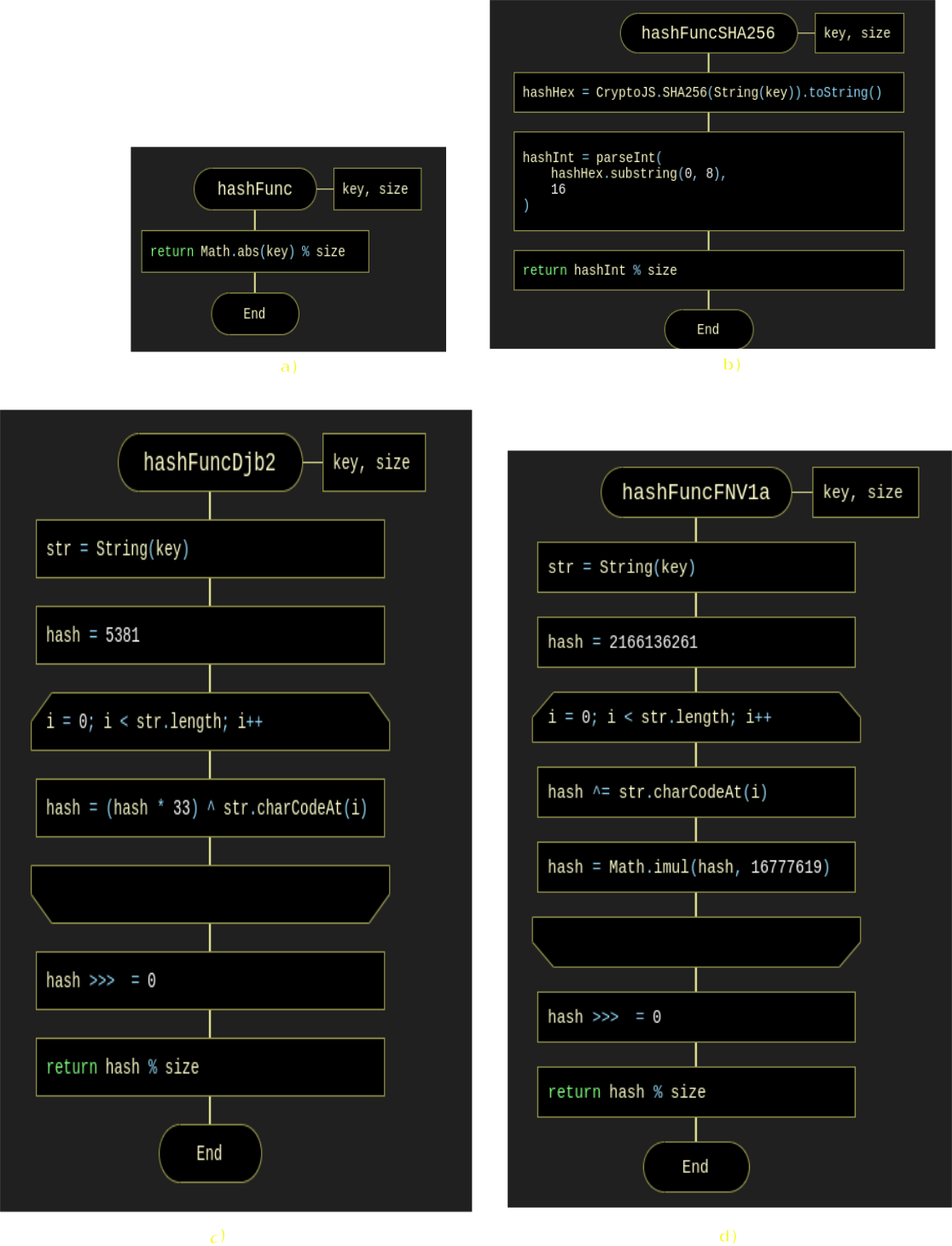
Figure 6.5. DRAKON-diagram of Hash Function Construction Methods

The simplest is the division method, where the hash is the remainder of the key divided by the number of buckets:

h(key) = key mod m (assuming the key is an integer).

In JavaScript, for numeric keys, this becomes h = x % m.

6.4.1. Creating a Hash Table and Chain Nodes

To implement a hash table using chaining, we need two helper structures: the table itself (an array of buckets) and a node for the linked list.

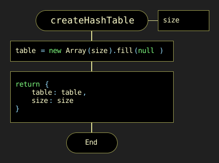
The function createHashTable(size) initializes a new hash table instance. It takes one argument – the desired number of buckets. Internally, it does the following (Figure 6.6):

Creates an array table of the given length.
Fills each element of the array with null. This means all buckets are initially empty – no key has been added yet.
Returns an object containing table and size. This object will be used by all subsequent operations (insert, traverse, lookup, remove).

In practice, the table object often also includes a count field (current number of elements) and a loadFactor (threshold for resizing). However, we start with a minimal version for simplicity.

Figure 6.6. Function for Creating a Hash Table (createHashTable)

Because collisions are resolved with linked lists, each element in a bucket must store not only a key‑value pair but also a reference to the next element in the same chain.

The function createNode(key, value, next = null) creates such a node (Figure 6.7). It:

Accepts a key, a value, and an optional reference to the next node (default null).
For debugging, prints a message to the console indicating that a node has been created. In production code this log is usually removed, but in educational examples it helps trace the algorithm’s behavior.
Returns an object with three fields: key, value, and next.

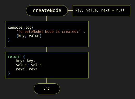
Figure 6.7. Function for Creating a Node (createNode)

Note that the next reference allows us to build singly linked lists inside a bucket. If only one element exists in a bucket, its next is null. When we add a new element that hashes to the same index, we place it at the beginning (or end – depending on the strategy; our algorithm will add to the head for simplicity).

As a result, this hash table would have as many singly linked lists (buckets) as specified by the Size constant. In the example below, the number of slots is 15.

Consider constructing a hash table of size m = 15 for a collection of integers from 0 to 119. The hash table slots are initially empty:

A hash function that establishes a relationship between an element and its corresponding slot must accept any element from the dataset (ranging from 0 to 119) and return an integer that corresponds to a slot number between 0 and 14. The algorithm implementing the remainder method sequentially processes each element from the original set, dividing it by 15 and returning the remainder as the hash value. This can be expressed as h(item) = item mod 15. For instance, the hash code for the element 119 is calculated as 119 mod 15 = 14 (since 119 - 15 × 7 = 14), thus placing the value 119 into the corresponding slot.

0	1	2	3	4	5	6	7	8	9	10	11	12	13	14
-	-	-	-	-	-	-	-	-	-	-	-	-	-	119

The algorithm then identifies slots for other elements, gradually filling them. When the algorithm encounters element 104 in the loop, the remainder of the division is 104 % 15 = 14, so this element will also be included in the 14th slot. In this way, each slot will accumulate corresponding elements with the same hash index. For example, for a hash index of 8, the slot will consist of these elements: 113, 98, 83, 68, 53, 38, 23, 8. The entire hash table will be as follows (Table 6.1):

Table 6.1: Hash Table of 15 Slots

0	1	2	3	4	5	6	7	8	9	10	11	12	13	14
105	106	107	108	109	110	111	112	113	114	115	116	117	118	119
90	91	92	93	94	95	96	97	98	99	100	101	102	103	104
75	76	77	78	79	80	81	82	83	84	85	86	87	88	89
60	61	62	63	64	65	66	67	68	69	70	71	72	73	74
45	46	47	48	49	50	51	52	53	54	55	56	57	58	59
30	31	32	33	34	35	36	37	38	39	40	41	42	43	44
15	16	17	18	19	20	21	22	23	24	25	26	27	28	29
0	1	2	3	4	5	6	7	8	9	10	11	12	13	14

Thus, the remainder method converts a collection of 120 integers into a hash table of 15 slots. The search for an element is now greatly accelerated as it takes two steps: first, the hash function h = (x % m) computes the hash index, and then the search is performed within a bucket (exactly 8 elements in each bucket for this example).

The implementation of the basic hash table functions using the hash function is as follows:

Create a HashTable structure of size m to store objects.
Compute the object’s hash code by passing it through the hash function.
Obtain the bucket hash indices where the objects will be stored.
Store these objects in the designated bucket.

The general description of algorithms for working with hash tables is presented as a table of basic parameters of applied functions (Table 6.2) and corresponding DRAKON diagrams (Figure 6.8a - 6.8f).

Table 6.2: Functions Overview (Chaining Implementation)

Function Purpose Parameters Return value Main steps Notes / Complexity

Function	Purpose	Parameters	Return value	Main steps	Notes / Complexity
`hashGet(hash, key)` (Figure 6.8a)	Find a value by key	`hash` – table object, `key` – search key	Value or `undefined` if not found	1. Compute index via `hashFunc`. 2. Traverse the chain at that bucket. 3. If `node.key === key` found, return `node.value`. 4. Otherwise return `undefined`.	Average-case (expected) O(1) complexity.
`hashInsert(hash, key, value)` (Figure 6.8b)	Insert or update a key‑value pair	`hash`, `key`, `value`	Bucket index where insertion/update occurred	1. Compute index. 2. Traverse the chain: if key exists, update its value and return index. 3. Otherwise, create a new node and insert at the head: `hash.table[index] = createNode(key, value, hash.table[index])`.	Insertion at the head is simpler and faster than at the tail.
`hashLookupByValue(hash, value)` (Figure 6.8c)	Find a key by value (reverse lookup)	`hash`, `value` – search value	Key or `undefined` if not found	1. Iterate over all buckets (0 to `size-1`). 2. In each bucket, traverse the chain. 3. If `node.value === value`, return `node.key`. 4. If not found, return `undefined`.	O(n) complexity – inefficient; use only for debugging or rare cases.
`hashRemove(hash, key)` (Figure 6.8d)	Delete an entry by key	`hash`, `key` – key to delete	`true` if deleted, `false` if key not found	1. Compute index. 2. Traverse the chain with a `prev` pointer. 3. If `node.key === key`: if `prev === null` (head) – `hash.table[index] = node.next`, else `prev.next = node.next`. 4. Return `true`. 5. If not found, return `false`.	The parameter must be `key`, not `value`.
`hashTraverse(hash)` (Figure 6.8e)	Print table contents (values only)	`hash`	– (console output)	For each bucket, print `"Slot i:"` followed by all values (`node.value`) separated by `" → "`, or `"Empty"` if the bucket is empty.	Does not show keys – `printHashTable` is more informative.
`printHashTable(hash)` (Figure 6.8f)	Print table in `key → value` format	`hash`	– (console output)	For each bucket, build an array of strings `"key → value"` for all nodes in the chain, then print joined by `" → "` or `"Empty"`.	Better than `hashTraverse` for debugging.

hashGet(hash, key) (Figure 6.8a)

Find a value by key

hash – table object, key – search key

Value or undefined if not found

1. Compute index via hashFunc.
2. Traverse the chain at that bucket.
3. If node.key === key found, return node.value.
4. Otherwise return undefined.

Average-case (expected) O(1) complexity.

hashInsert(hash, key, value) (Figure 6.8b)

Insert or update a key‑value pair

hash, key, value

Bucket index where insertion/update occurred

1. Compute index.
2. Traverse the chain: if key exists, update its value and return index.
3. Otherwise, create a new node and insert at the head:
hash.table[index] = createNode(key, value, hash.table[index]).

Insertion at the head is simpler and faster than at the tail.

hashLookupByValue(hash, value) (Figure 6.8c)

Find a key by value (reverse lookup)

hash, value – search value

Key or undefined if not found

1. Iterate over all buckets (0 to size-1).
2. In each bucket, traverse the chain.
3. If node.value === value, return node.key.
4. If not found, return undefined.

O(n) complexity – inefficient; use only for debugging or rare cases.

hashRemove(hash, key) (Figure 6.8d)

Delete an entry by key

hash, key – key to delete

true if deleted, false if key not found

1. Compute index.
2. Traverse the chain with a prev pointer.
3. If node.key === key:
if prev === null (head) – hash.table[index] = node.next,
else prev.next = node.next.
4. Return true.
5. If not found, return false.

The parameter must be key, not value.

hashTraverse(hash) (Figure 6.8e)

Print table contents (values only)

hash

– (console output)

For each bucket, print "Slot i:" followed by all values (node.value) separated by " → ", or "Empty" if the bucket is empty.

Does not show keys – printHashTable is more informative.

printHashTable(hash) (Figure 6.8f)

Print table in key → value format

hash

– (console output)

For each bucket, build an array of strings "key → value" for all nodes in the chain, then print joined by " → " or "Empty".

Better than hashTraverse for debugging.

DRAKON-diagrams of hash table algorithms: find by key, insert, reverse lookup, delete, traverse, and print are shown in Figure 6.8a–f.

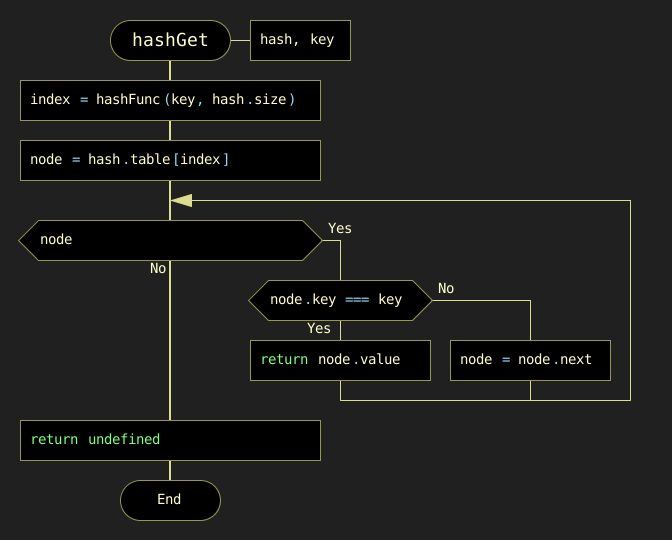
Figure 6.8a. Hash Table Search by Key (hashGet)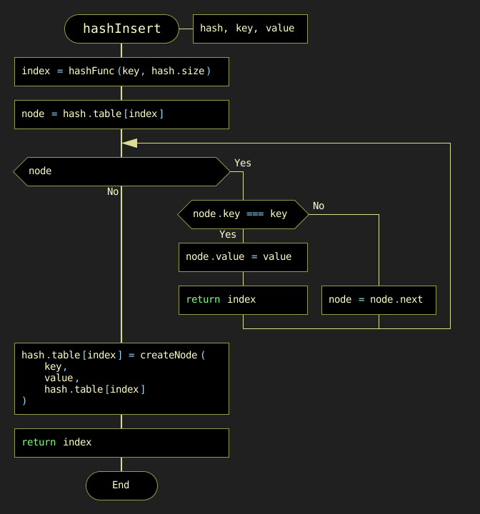

Figure 6.8b. Hash Table Insertion or Update (hashInsert)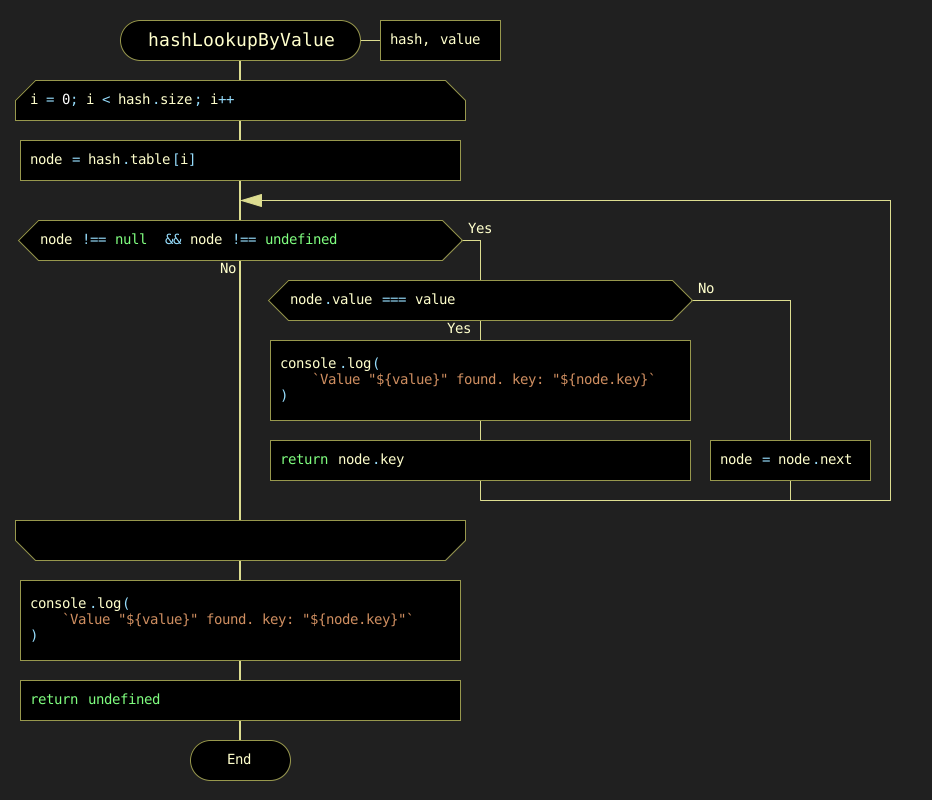

Figure 6.8c. Hash Table Reverse Lookup by Value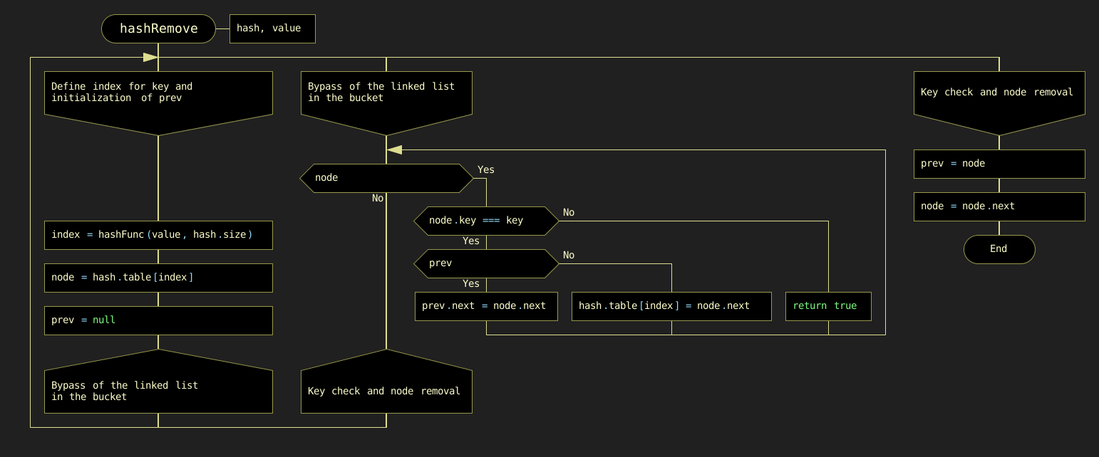 (hashLookupByValue)

Figure 6.8d. Hash Table Deletion by Key (hashRemove)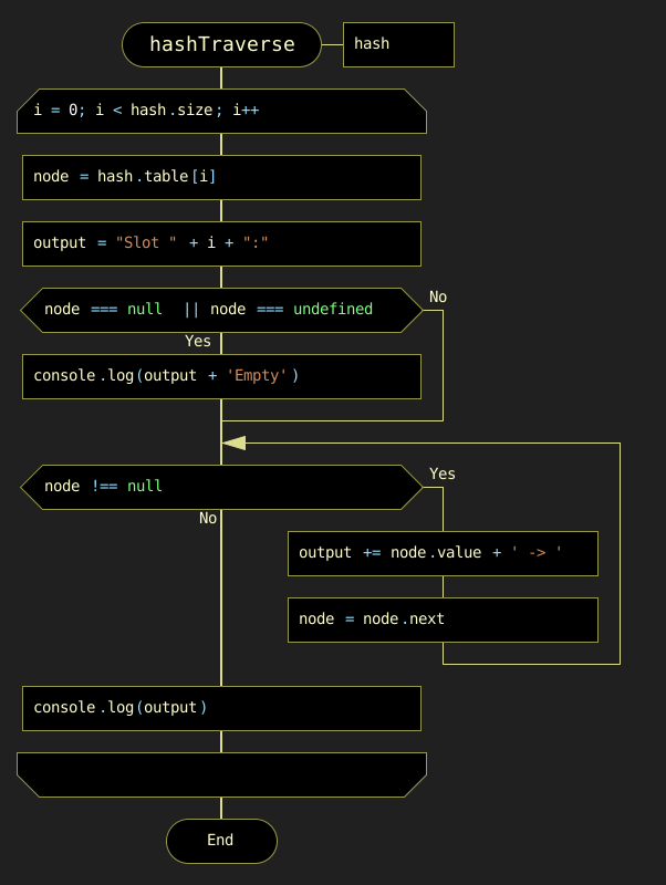

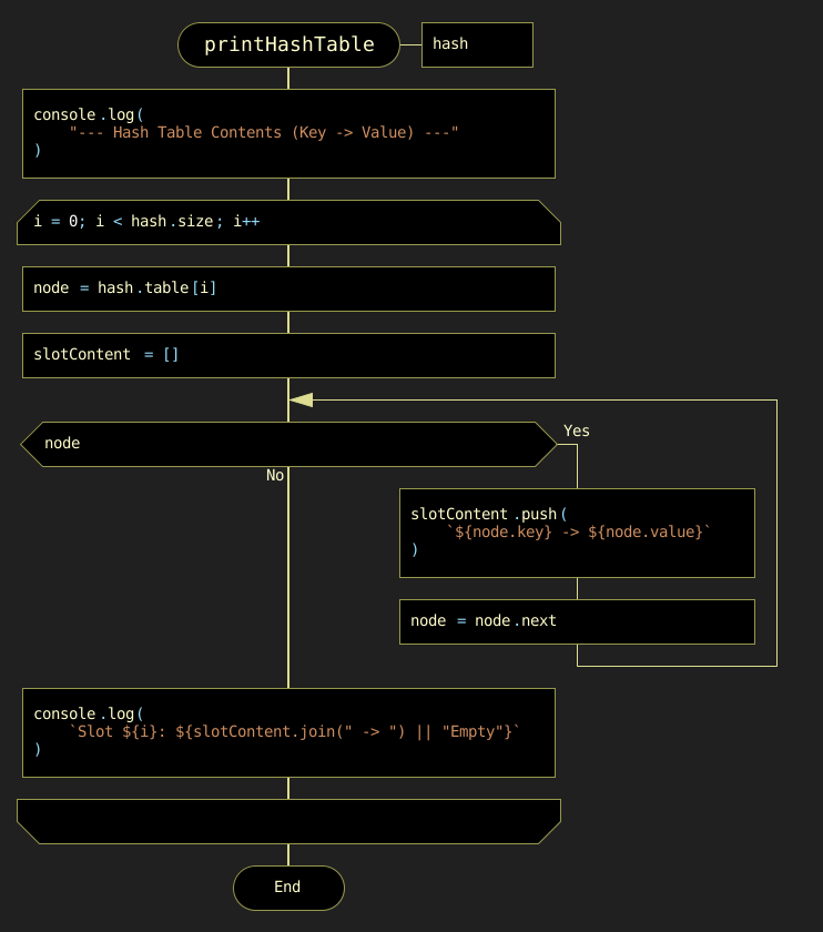
Figure 6.8e. Hash Table Traversal Function (hashTraverse)

Figure 6.8f. Hash Table Printing (printHashTable)

6.4.2. Concrete Example

Consider a concrete example. A hash table of size m = 16 is populated with 16 records, each keyed by a six-digit identifier and holding a person’s name as the value. Calling printHashTable(hash) after all insertions produces the following snapshot of the table (Table 6.3):

Table 6.3: Hash Table Contents Before Removal (printHashTable, m = 16)

Slot	Chain (key → value)
0	Empty
1	625073 → Olivia J. Watson
2	Empty
3	519283 → Alice R. Cooper
4	476820 → Ivy N. Butler → 357908 → Carol A. Foster
5	807541 → Mia G. Richardson → 392645 → Jack K. Barnes → 430165 → Emma L. Reed
6	941206 → Paul V. Steven → 746102 → Bob M. Bennett
7	Empty
8	679832 → Frank W. Brooks
9	Empty
10	169834 → Noah D. Patterson → 734218 → Leo C. Coleman → 821674 → David S. Hughes
11	213547 → Grace E. Simmons
12	Empty
13	958301 → Henry T. Peterson
14	Empty
15	568079 → Kelly P. Ross

Suppose we now call hashRemove(hash, 821674). The algorithm proceeds as follows:

Compute the bucket index: hashFunc(821674) = 821674 mod 16 = 10.
Traverse the chain stored in slot 10. The chain currently holds three nodes: 169834 → Noah D. Patterson, 734218 → Leo C. Coleman, 821674 → David S. Hughes.
After each node.key === key check, the previously visited node is kept in the prev variable. The first two nodes (169834, 734218) do not match and are skipped in turn.
The third node matches (node.key === 821674). Since it is not the head of the chain, the link is repaired by setting prev.next = node.next — the node holding David S. Hughes is detached from the chain, and hashRemove returns true.

Only slot 10 is affected by this operation; every other slot remains exactly as in Table 6.4:

Table 6.4: Slot 10 Before and After hashRemove(hash, 821674)

State	Chain (key → value)
Before	169834 → Noah D. Patterson → 734218 → Leo C. Coleman → 821674 → David S. Hughes
After	169834 → Noah D. Patterson → 734218 → Leo C. Coleman

State

Chain (key → value)

Before

169834 → Noah D. Patterson → 734218 → Leo C. Coleman → 821674 → David S. Hughes

After

169834 → Noah D. Patterson → 734218 → Leo C. Coleman

Finally, consider a call to hashLookupByValue(hash, "Olivia J. Watson") — a reverse lookup, illustrating the O(n) traversal described in Table 6.2. The algorithm scans every bucket in order; the very first non-empty bucket it inspects, slot 1, already contains the matching node, and the function returns key 625073. Unlike hashGet, which locates a value in average-case O(1) time by jumping straight to the correct bucket, hashLookupByValue has no such shortcut: in the worst case it must inspect every node in every bucket before concluding that no match exists.

Topics Beyond the Scope of This Book

This section has focused on the fundamental principles of hashing and the implementation of a hash table using separate chaining. However, several important and advanced aspects of modern hashing remain outside the scope of this book:

Open addressing techniques — linear probing, quadratic probing, and double hashing.
Dynamic resizing of hash tables when the load factor exceeds a threshold.
Cryptographic hash functions (MD5, SHA family, etc.) used for data integrity and security rather than indexing.
Perfect hashing and minimal perfect hashing, which eliminate collisions entirely but require complex precomputation.
Distributed hash tables (DHTs) — used in peer-to-peer networks and blockchain architectures.

These topics will be explored in future works devoted to large-scale data management, high-performance systems, and secure information storage.

Computational Experiment

The user enters an array and a target value, or selects "Random sorted array" / "Random unsorted array".

Before execution, they can predict whether Binary Search will locate the target.

Clicking "Run all searches" executes all three algorithms against the same dataset.

A results table displays the output and the number of comparisons made by each algorithm, followed by a step-by-step trace (low, mid, high pointers for Binary Search).

If the array is unsorted, a warning is raised. If Binary Search fails to find an existing target due to the lack of sorting, the page explicitly highlights this behavior.

Run experiment

0	1	2	3	4	5	6	7	8	9	10	11	12	13	14
105	106	107	108	109	110	111	112	113	114	115	116	117	118	119
90	91	92	93	94	95	96	97	98	99	100	101	102	103	104
75	76	77	78	79	80	81	82	83	84	85	86	87	88	89
60	61	62	63	64	65	66	67	68	69	70	71	72	73	74
45	46	47	48	49	50	51	52	53	54	55	56	57	58	59
30	31	32	33	34	35	36	37	38	39	40	41	42	43	44
15	16	17	18	19	20	21	22	23	24	25	26	27	28	29
0	1	2	3	4	5	6	7	8	9	10	11	12	13	14

0	1	2	3	4	5	6	7	8	9	10	11	12	13	14
105	106	107	108	109	110	111	112	113	114	115	116	117	118	119
90	91	92	93	94	95	96	97	98	99	100	101	102	103	104
75	76	77	78	79	80	81	82	83	84	85	86	87	88	89
60	61	62	63	64	65	66	67	68	69	70	71	72	73	74
45	46	47	48	49	50	51	52	53	54	55	56	57	58	59
30	31	32	33	34	35	36	37	38	39	40	41	42	43	44
15	16	17	18	19	20	21	22	23	24	25	26	27	28	29
0	1	2	3	4	5	6	7	8	9	10	11	12	13	14

0	1	2	3	4	5	6	7	8	9	10	11	12	13	14
105	106	107	108	109	110	111	112	113	114	115	116	117	118	119
90	91	92	93	94	95	96	97	98	99	100	101	102	103	104
75	76	77	78	79	80	81	82	83	84	85	86	87	88	89
60	61	62	63	64	65	66	67	68	69	70	71	72	73	74
45	46	47	48	49	50	51	52	53	54	55	56	57	58	59
30	31	32	33	34	35	36	37	38	39	40	41	42	43	44
15	16	17	18	19	20	21	22	23	24	25	26	27	28	29
0	1	2	3	4	5	6	7	8	9	10	11	12	13	14