Section 8. Binary Tree Algorithms

This section presents an advanced study of binary tree data structures and algorithms, spanning Binary Search Trees (BST), AVL trees, and Red-Black Trees (RBT), implemented using JavaScript and visual programming formalisms (DRAKON diagrams). A key contribution of this work is the author’s innovative conceptual framework based on a node cluster (C-Cluster) representation for insertion and deletion operations. Within this model, the local spatial topology, color state, and structural relationships of candidate nodes are encoded into a compact character string (a textual cluster descriptor). This information image abstracts complex pointers and significantly simplifies the conditional logic of tree restructuring algorithms. Furthermore, this section introduces a novel mechanical analogy for Red-Black Tree balancing—modeling the structure as a suspended chandelier governed by gravitational equilibrium, where black nodes act as solid unit weights and red nodes act as weightless spacers. This mechanical paradigm renders abstract invariants (such as uniform black height and double-red prevention) visually intuitive and directly translates into the automated decision rules of a virtual balancing automaton. Additionally, the section covers foundational traversal strategies, canonical rotation primitives (LL, RR, LR, RL), and exact complexity trade-offs, providing both theoretical rigor and a complete visual reference framework.

8.1. Representation of Binary Trees

A binary tree is a hierarchical data structure in which each node has at most two children, referred to as the left and right child. The topmost node is called the root, and nodes with no children are called leaves.

Binary trees as an abstract data type were discussed in Section 1. Here we will discuss the computer implementation of this type of data structure using the visual algorithmic language DRAKON and the JavaScript programming language. Recall the basic terminology of binary trees (Figure 8.1):

Figure 8.1. Basic tree terminology

Root: The root of the tree is the only node with no incoming edges. It is the top node in the tree.
Node: The basic element of the tree. Each node has data and two references that can point to zero or more children.
Edge: A fundamental part of the tree used to connect two nodes.
Path: An ordered list of nodes connected by edges.
Leaf: A leaf node is a node that has no children.
Tree height: The number of edges on the longest path between the root and a leaf.

Node level: The number of edges on the path from the root node to that node.

The information structure of a binary tree is organized as follows (Figure 8.2):

Figure 8.2. Binary tree structure

Several types of binary trees are discussed in the literature, the most important classification being based on node values:

Binary Search Tree (BST)
AVL Tree (Adelson-Velsky and Landis Tree)
Red-Black Tree

8.2. Binary Search Tree

8.2.1. Building a Binary Tree

If the tree is organized such that, for each node, all node values of its left subtree are less than this node and all values of its right subtree are greater, it is called a binary search tree (BST). A BST is a recursive data structure because each subtree is also a tree. A BST has the following properties:

Each node retains a unique value.
Each node has zero, one, or two child nodes.
One node is referred to as the root node, which is at the top of the tree structure.
Each node has only one parent node, except for the root node which has no parent.
The value of each node is greater than that of its left child but less than that of its right child.

A binary search tree is built according to a specific algorithm. Consider the sequence of integers {11, 5, 17, 15, 1, 8, 19, 13, 21}, represented as a slice of numbers. First the root node {11} is formed, then in a loop for each node the method insertNode(tree, value) is called recursively (Figure 8.3a), which in turn calls the method createNode(value), which creates a new node (Figure 8.3b) in the resulting tree (Figure 8.3c).

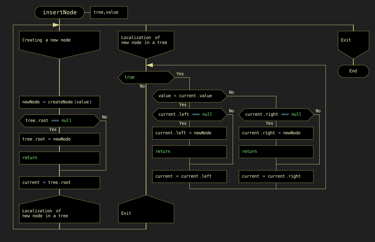
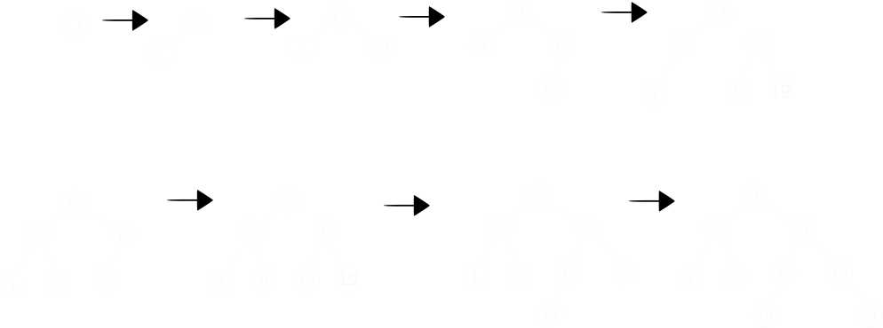
Figure 8.3. Binary tree DRAKON-diagrams: a) building a tree by insert(node, value); b) creating a node

The complete process of creating a binary tree is shown in Figure 8.4. The first number 11 is written to the root of the tree. The second number 5 is less than the value in the tree root, so it is written to the left subtree. The next number 17 is greater than the root number, so it is written to the right subtree. Then the number 15 is greater than the value at the root of the tree, so it is written to the right subtree, but the right subtree is already built. The number 15 is compared to the number 17 at the root of the right subtree. Since the value to be added is less than the value in the root of the right subtree, we add the left subtree to this node. The final result is a binary search tree with three variants: node 5 is the parent of two children (1, 8), node 15 has only a left child, and node 19 has only a right child. This arrangement of nodes is chosen to demonstrate the node removal function, which will be discussed later.

Figure 8.4. Building a binary tree

8.2.2. Finding a Node Based on a Given Value

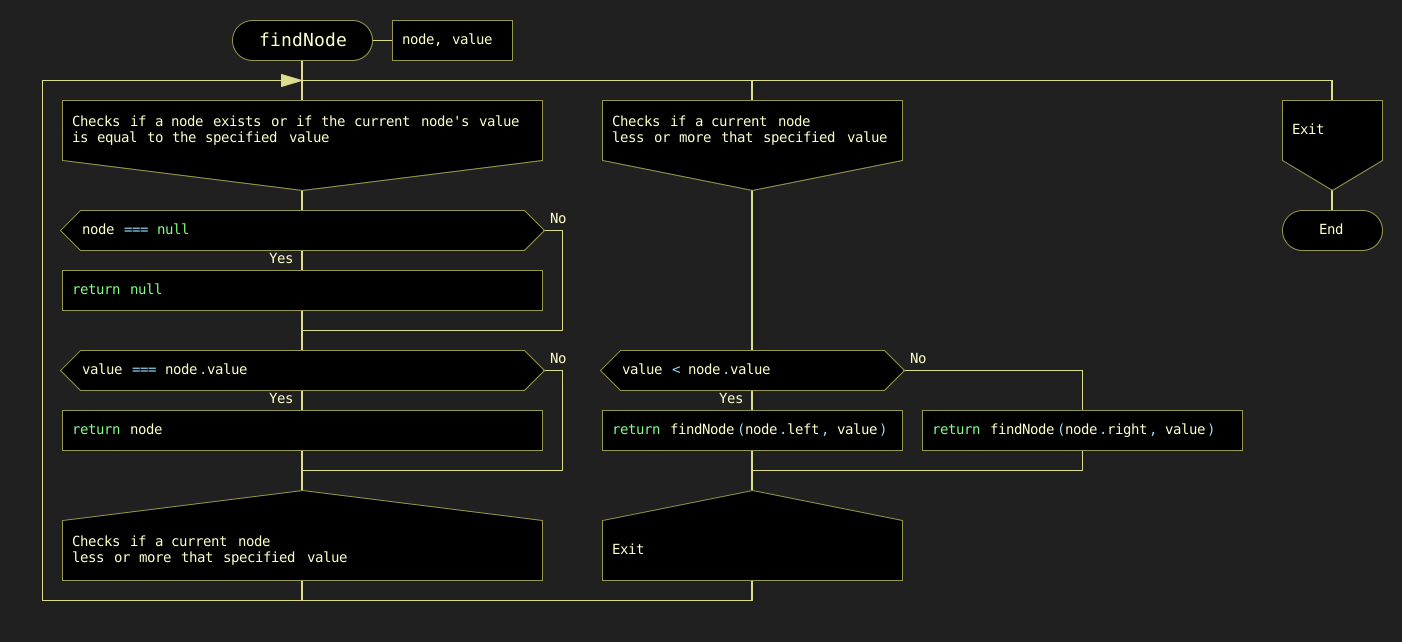
Another basic operation is the findNode(value) function. This function uses a JavaScript construct that recursively compares the value of val with the values of other nodes as it traverses the tree. The DRAKON-diagram of the findNode(node, value) function is shown in Figure 8.5.

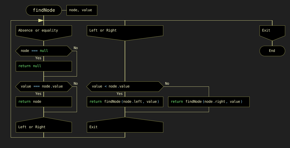
Figure 8.5. DRAKON-diagram of the node finding algorithm

8.2.3. Deleting a Node with a Specified Value

The next basic operation is deleting a node with a specified value. The function removeNode(node, value) is used recursively.

Let us analyze in more detail the order in which nodes are moved in these variants.

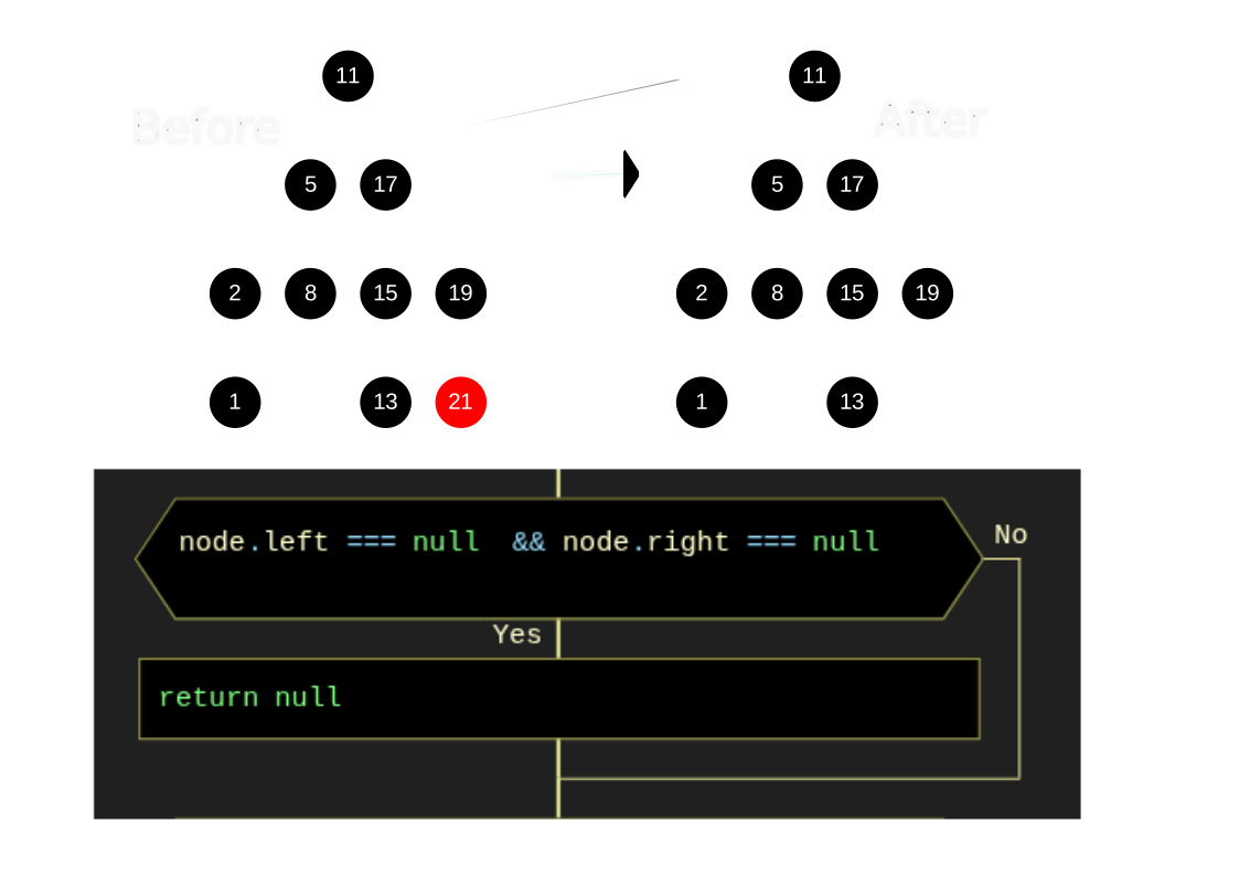
Option a): Node (21) has no children (Figure 8.6).

In this case, this node is removed by changing the value of node = null in the parent node. Figure 8.6 shows the process of deleting node (21) and the corresponding DRAKON-diagram fragment.

Figure 8.6. Deleting a node without children

Option b): Node (19) has a right child (Figure 8.7).

In this case, node (19) is removed from the tree by replacing its address in the parent node (17) with the address of its only child node (21). Figure 8.7 shows the process of removing node (19) and the corresponding DRAKON-diagram fragment.

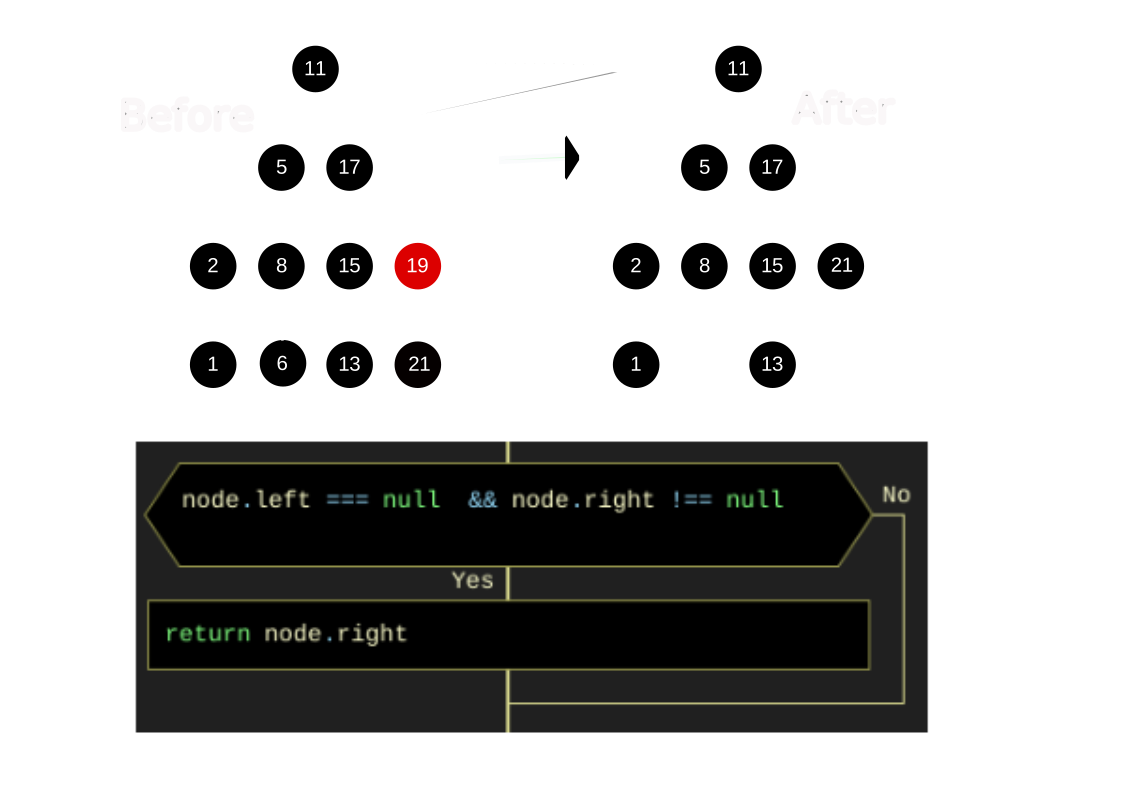
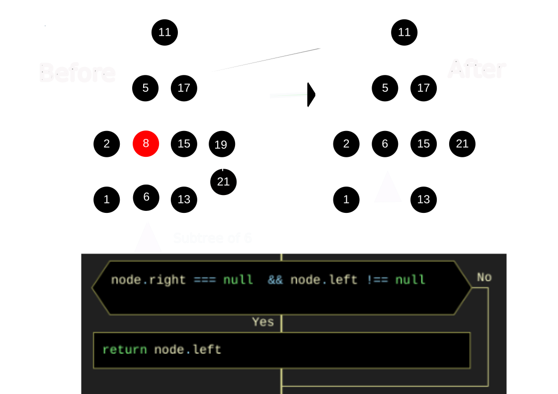
Figure 8.7. Deleting node (19) with a right child

Option c): Node (8) has a left child (Figure 8.8).

In this case, node (8) is removed from the tree by replacing its address in parent node (5) with the address of its only left child node (6). Figure 8.8 shows the process of removing node (8) and the corresponding DRAKON-diagram fragment.

Figure 8.8. Deleting node (8) with a left child

Option d): Node (5) has two children (Figure 8.9). In this case the binary search tree is rearranged: node (2) moves to the place of node (5).

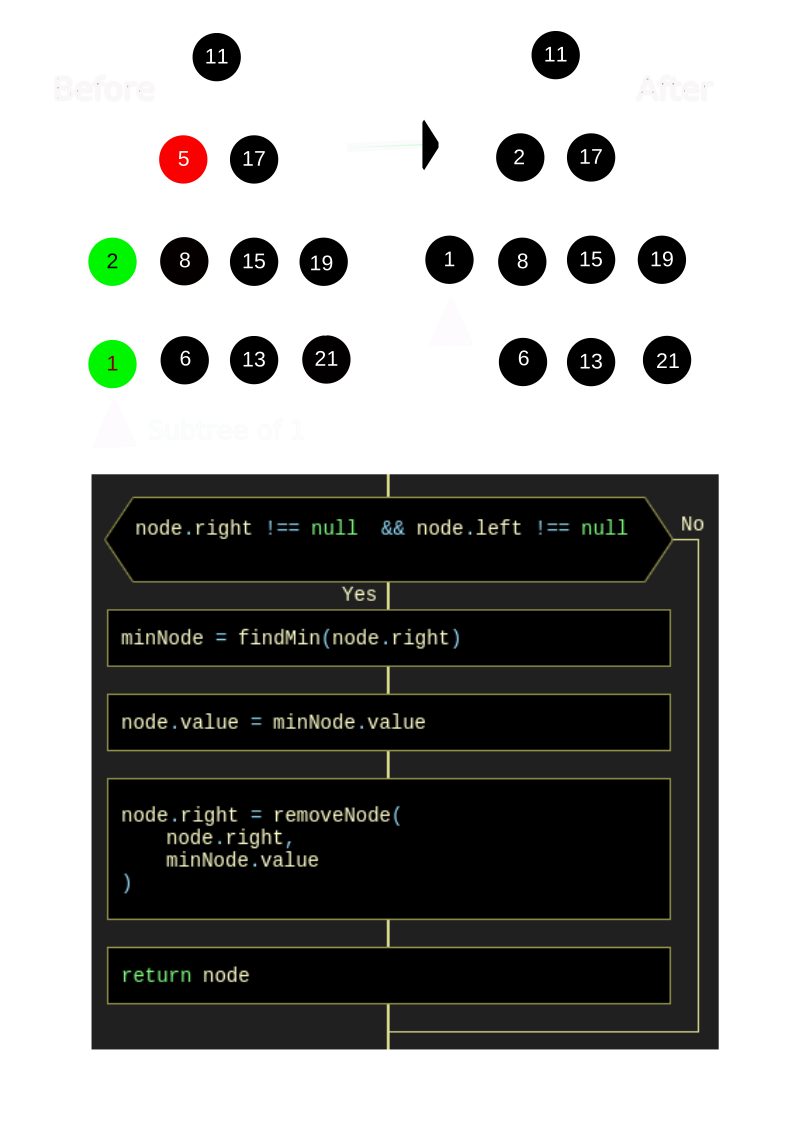
Figure 8.9. Deleting node (5) with two children

The DRAKON-diagram of the minimum value search method is shown in Figure 8.10.

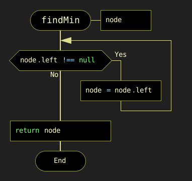
Figure 8.10. DRAKON-diagram of the minimum value search method

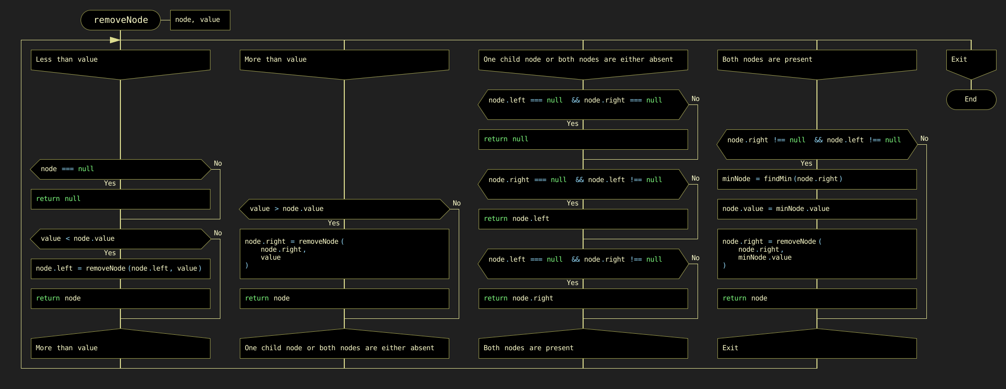
The complete DRAKON-diagram of node removal from a binary search tree is shown in Figure 8.11.

Figure 8.11. DRAKON-diagram of node removal

8.2.4. Traversing the Binary Search Tree

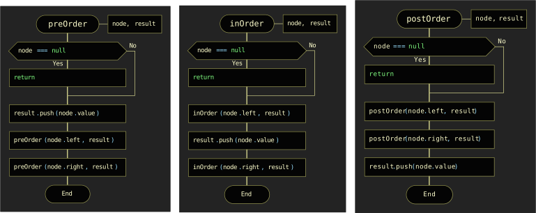
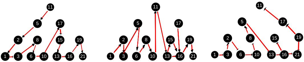
One of the basic tree operations is traversing tree nodes. Unlike linear data structures, where elements are traversed in a linear order, tree nodes can be traversed in a variety of ways.

Pre-order walk: Each ancestor node is visited before its descendants.
In-order walk: The left subtree is visited from bottom to top, then the root node, then the right subtree.
Post-order walk: Descendants are visited first, then ancestors.

All three cases, including the DRAKON diagrams, are shown in Figure 8.12.

Figure 8.12. Three classical tree traversals: Pre-, In-, and Post-order

Computational Experiment

Enter a sequence of integer values, construct a binary search tree, and observe its structure before and after deleting a selected node.

Run experiment

8.3. Self-Balancing Binary Trees (AVL Trees)

The efficiency of binary tree processing algorithms significantly depends on the order in which node values are provided during tree construction. In the most favorable sequence, the binary tree becomes balanced. In the worst-case sequence, the "tree" degenerates into a "branch" (Figure 8.13). As we will see below, restoring balance in such cases reduces to four canonical rotation patterns — right, left, right-left, and left-right rotation.

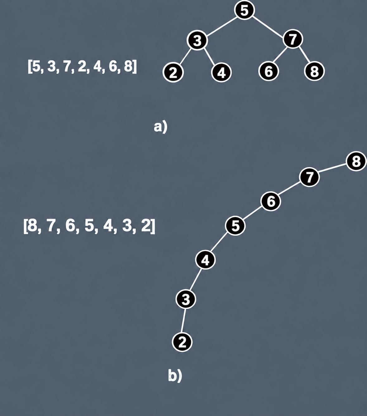
Figure 8.13. Most favorable (a) and worst-case (b) input data sequences

In such practically "degenerate" trees, the complexity of operations is determined by the number of nodes — that is, it is almost linear: O(n). The left and right subtrees are unbalanced, which can be estimated by the balance factor (bf), which is equal to the difference between the heights of the left and right subtrees. Recall that the height of a tree is defined as the length of the longest branch in a subtree (sum of edges). For an ideal binary search tree (a tree where the number of nodes in the left subtree equals the number of nodes in the right subtree), this factor is 0 (Figure 8.14).

Figure 8.14. An ideal binary tree

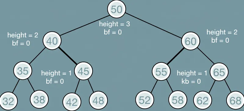
In real life, ideal binary trees are almost never achieved. Programmers often try to build a tree where the height of the left subtree differs from the height of the right subtree by no more than 1. Such trees are called AVL trees; for these trees the complexity of operations is defined as O(log n), meaning the execution time of basic operations (search, delete) is significantly less than for BST trees.

The algorithms for such trees are based on the process of balancing the tree when a new node is inserted or an existing node is removed. The purpose of balancing is to reconstruct the tree so that the heights of the left and right subtrees do not differ by more than 1. The balance factor must satisfy the following conditions:

The allowable values are bf = -1, 0, and +1.
bf = -1 indicates that the right subtree "outweighs" the left subtree.
bf = +1 indicates that the left subtree "outweighs" the right subtree.
bf = 0 indicates that the tree contains an equal number of nodes on each side — that is, the tree is perfectly balanced.

The balancing algorithm in its most general form is presented in the following DRAKON diagram (Figure 8.15):

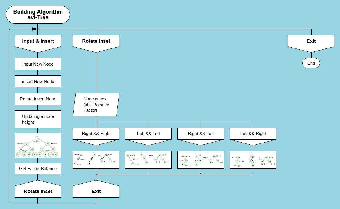
Figure 8.15. The balancing algorithm in its most general view

The balancing technique boils down to making circular movements of the nodes in four variants:

Right rotation (RR)
Left rotation (LL)
Right-left rotation (RL)
Left-right rotation (LR)

Right rotation is performed when the root node has a balance factor bf = +2 and its left child has a balance factor bf = +1 (Figure 8.16):

Figure 8.16. Right rotation

Left rotation is performed when the root node has a balance factor bf = -2 and its right child has a balance factor bf = -1 (Figure 8.17):

Figure 8.17. Left rotation

Right-left rotation is performed when the root node has a balance factor bf = -2 and its right child has a balance factor bf = +1 (Figure 8.18):

Figure 8.18. Right-left rotation

Left-right rotation is performed when a node has a balance factor bf = +2 and its left child has a balance factor bf = -1 (Figure 8.19):

Figure 8.19. Left-right rotation

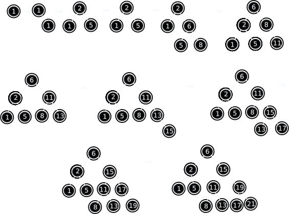
Consider the balancing process in more detail with an example of tree formation when input data is received in this order: [1, 2, 5, 6, 8, 11, 13, 15, 17, 19, 21]. As shown above, such a tree is unbalanced.

Balance checks are started on the arrival of each new node using the insertNode(node, value) function, which determines the position of the new node in the left or right subtree relative to the root node. The choice of the balancing path is determined by the method rotateInsert(node, value). A DRAKON-diagram of the algorithms of the above methods is shown in Figure 8.20.

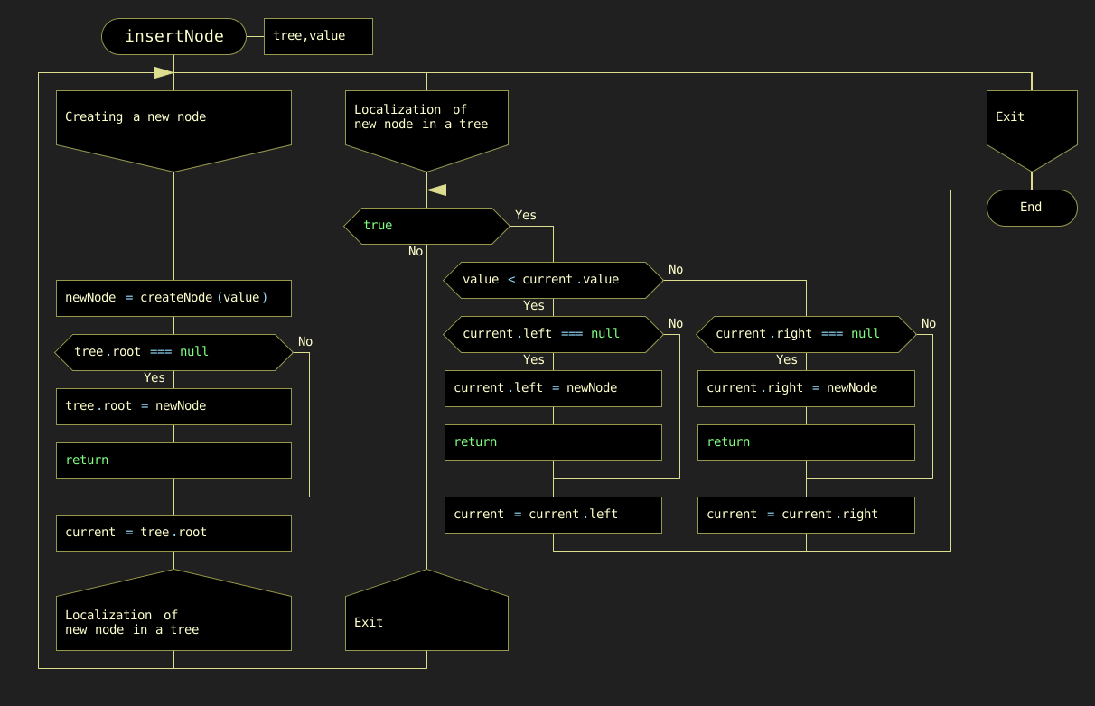
Figure 8.20. DRAKON-diagram depicting the method of inserting a node

The choice of one of the possible balancing paths (rotations) is determined by the rotateInsert(node, val) function (Figure 8.21).

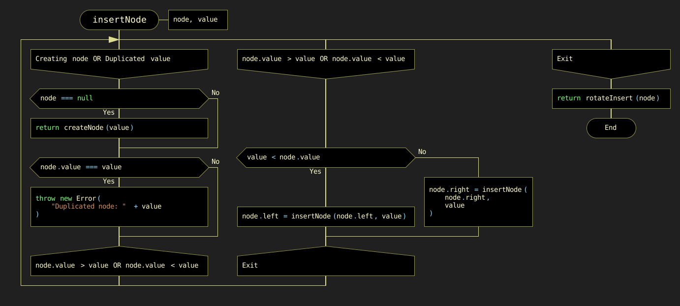
Figure 8.21. DRAKON-diagram depicting the rotation selection method

Depending on the location of the new node relative to the parent node and the balance factor values, the left-hand or right-hand rotation methods are performed (Figure 8.22):

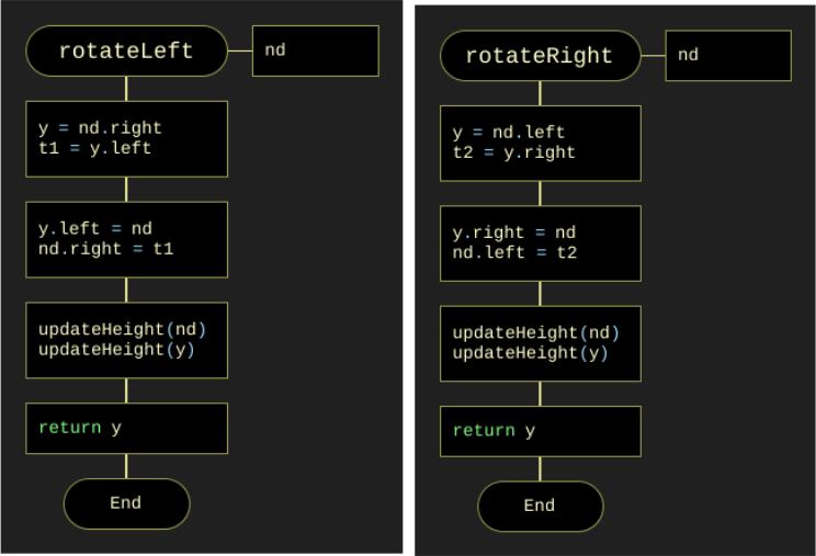
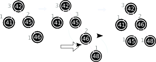
Figure 8.22. Node rotation program codes

Let us examine the tree rebuilding process in detail as a result of using the rotateInsert(node, val) method on the example of entering the values of three nodes (5, 6, 8). After receiving the value of the last node (8), a "twig" appears instead of a tree that needs to be balanced. In this case the condition in the rotateInsert(node, val) method is met: the balancing factor is 2 (bf = 2) and the value of node (8) is greater than the parent node (6), so the rotateLeft(node) method is called. The balancing process in this case is shown in Figure 8.23:

Figure 8.23. Example of left-left rotation balancing

The process of new nodes arriving and rebuilding the resulting AVL tree by balancing for the input set [1, 2, 5, 6, 8, 11, 13, 15, 17, 19, 21] is shown in Figure 8.24.

Figure 8.24. Process of building a balanced AVL tree

The DRAKON-diagram of the AVL tree basic operation findNode(node, val) is shown in Figure 8.25:

Figure 8.25. DRAKON-diagram depicting the node finding method

Another basic operation, deleting a node with a specified value, consists of the following steps. The node is searched from the root down through the branches to the node to be deleted. The following situations may occur (Figure 8.26):

Figure 8.26. Cases for nodes to be removed

a) The node to be deleted has two non-empty children. b) The node to be deleted has no children. c) The node to be deleted has one child (left or right).

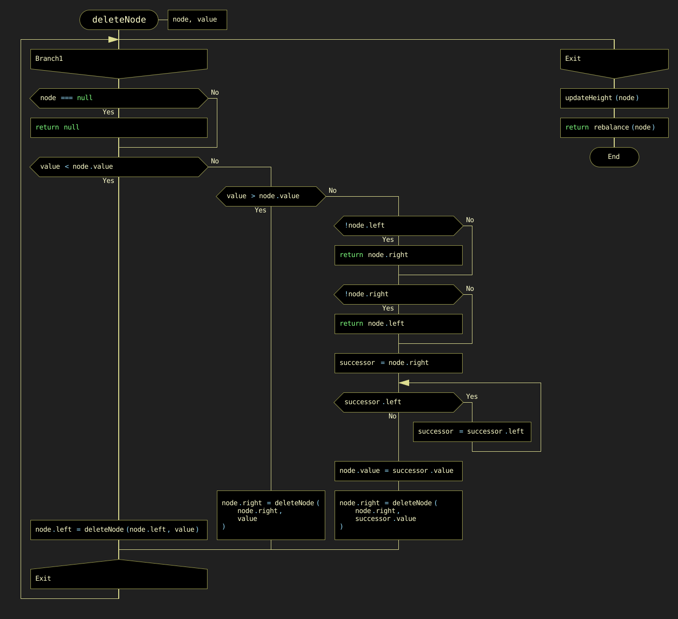
As with the other methods, a node with a given value is first recursively identified and then one of the options presented is selected. A DRAKON-diagram of the algorithm for deleting a node with a specified value is shown in Figure 8.27.

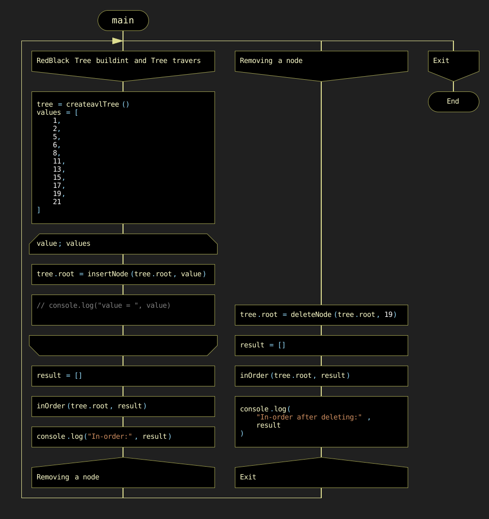
Figure 8.27. DRAKON-diagram depicting an algorithm for removing a node with a specified value

The main() program inputs an array of data, searches for a node with a specified value, and deletes a node with a specified value (Figure 8.28).

Figure 8.28. DRAKON-diagram of the main function

Computational Experiment

Enter a sequence of integer values, construct an AVL tree, and observe its structure before and after deleting a selected node.

More information about the experiment can be found in the App by activating the "Launch Sorting Experiment" button.

Run experiment

8.4. Red-Black Trees

8.4.1. Description of Red-Black Tree Properties as a Data Structure

A red-black tree is a variant of a self-balancing binary search tree in which the nodes are colored red or black according to a specific set of rules (Figure 8.29).

Figure 8.29. Red-black tree example

The nodes containing data (integers in this example) are called internal nodes. In addition, red-black trees contain imaginary "null" nodes associated with tree leaves, which are explicitly colored black (labeled "Null" in Figure 8.29). Red-black trees satisfy all properties of a binary search tree and must maintain the following specific invariants:

Each node is colored either red or black.
The root of the tree must be black. (Note: this invariant may be temporarily violated during the balancing process but must be restored before the operation completes.)
All leaves (NIL nodes) are black.
Both children of a red node must be black. Consequently, no two red nodes can appear consecutively on any path.
Every simple path from a node to any of its descendant leaves must contain the same number of black nodes.

Unlike AVL trees, where balance is enforced by limiting the height difference between subtrees, red-black tree balance is achieved by strictly enforcing the properties listed above. Inserting or removing a node can disrupt these invariants. Balance is restored using two primary operations: recoloring nodes and/or restructuring the tree (or subtrees) using specific rotations. The most critical of these constraints are Properties 4 and 5.

Property 4 mandates that two red nodes cannot be adjacent.
Property 5 builds on this by enforcing a uniform black height for all paths from any node to its leaf descendants. Regardless of the specific path taken, the count of black nodes remains constant.

Mechanical Analogy for Balancing: The Chandelier and the Balancing Machine

Understanding the dynamic enforcement of red-black properties is crucial for developing an efficient balancing algorithm. However, this often presents significant challenges, as it requires tracking the state of multiple nodes simultaneously.

To facilitate conceptual clarity, we employ a mechanical analogy. Since the "root" of this data structure is positioned at the top, a chandelier serves as an appropriate mechanical analogue — an elegant hanging structure where each node is a ball of a strictly defined color and weight, rigidly connected to form branches. The root is fixed at the top, and the weightless NIL leaves hang freely downward.

In this model:

Black balls are solid and heavy, providing stability and physical equilibrium. Their weight is defined as 1 unit.
Red balls are hollow, decorative, and virtually weightless (0 units). They serve as a flexible resource that can be "hardened" into black balls (weights) when necessary.

All NIL leaves are considered black and weightless termination points.

The structural equilibrium (balance) is defined by two simple conditions, which restate Properties 5 and 4 respectively in mechanical terms:

The total weight (the number of black balls) on any path from the root to any leaf must be equal — this is Property 5, the uniform black height.
Two red balls in a row are forbidden — this creates a "weak spot" in the chain, even though it does not alter the branch’s overall weight; this is Property 4.

Black height is the fundamental metric in this engineering model, representing the total "weight" (the number of black nodes) of a specific branch. Properties 4 and 5 work together to ensure structural integrity. While red nodes allow branches to stretch, the rules guarantee that the longest path (alternating black weights and red spacers) is never more than twice the length of the shortest path (consisting only of black weights). This constraint ensures that "tension" is evenly distributed, keeping the tree approximately balanced with a height of O(log n), where n is the number of nodes.

The entire lifecycle of the structure is managed by a virtual balancing automaton. It possesses an unlimited stock of spare black and red balls and performs four functions:

Insertion: The automaton hangs a new red ball (NIL replacement).
Deletion: It removes a ball and replaces it with a dummy, triggering rebalancing if necessary.
Balance Monitoring: After every insertion or deletion, it checks for equilibrium violations.
Balancing: If a violation is detected, the automaton performs local transformations: recoloring balls and/or rearranging connections (rotations) using its stock of spare parts.

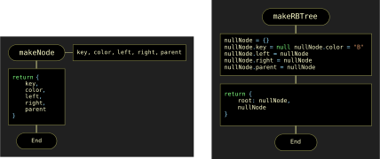
To implement these operations, we define two custom data types: node and rbTree. A node includes fields for the key (numeric value), color (boolean: true for red, false for black), and pointers to left, right, and parent nodes. The rbTree structure is a reference-type variable that stores a pointer to the memory area containing the tree objects (Figure 8.30).

Figure 8.30. DRAKON-diagram of Node and rbTree description

Cluster Node Notation

To analyze the balancing process, we introduce an original cluster-based notation, developed specifically for this book, which focuses on a local C-Cluster of nodes involved in a transformation. This notation is essential for understanding the transformations applied by the automaton. The following designations are used (Figure 8.31):

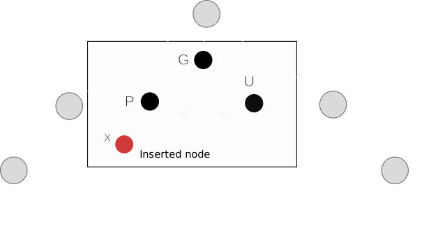
Figure 8.31. Designation of "kinship" degrees of RB tree nodes (Cluster x, P, G, U, S)

In this model:

x: The newly inserted red node.
P: Parent of x.
G: Grandparent of x (parent of P). In our model, G is always a solid 'weight' (black) before fixup begins.
U: Uncle of x (sibling of P). A missing (null) uncle is treated as a static black 'weight' (NIL leaf).
S: Sibling of x (the other child of P). Its color and position are crucial for determining the necessary rotation type.

For a compact description of the cluster arrangement, we introduce the following symbolic notation:

A colon : separates the node name from its color (P:B describes a black parent).
The comparison symbols < and > indicate relationship direction (x<P means x is `P’s left child).
Commas and semicolons delimit attributes.

For example, the notation x:R, x<P; P:R, P>G; G:B; U:R; U>G; describes a specific "zig-zag" violation where red node x is the left child of its red parent P, which in turn is the right child of the black grandparent G, who also has a red uncle U. Cluster nodes can be in a "zig-zig" (e.g., x<P<G) or "zig-zag" (e.g., x<P>G) configuration.

This concise notation significantly simplifies the balancing algorithms, making the transformation criteria visual and efficient.

8.4.2. Inserting a New Node and the Balancing Process

A new node is inserted into the red-black tree using the rbInsert(tree, key) function, which follows standard BST rules and always adds a new red node. However, this addition may introduce a "Double Red" conflict (violating Property 4). The rebalancing process is summarized in the mindmap in Figure 8.32.

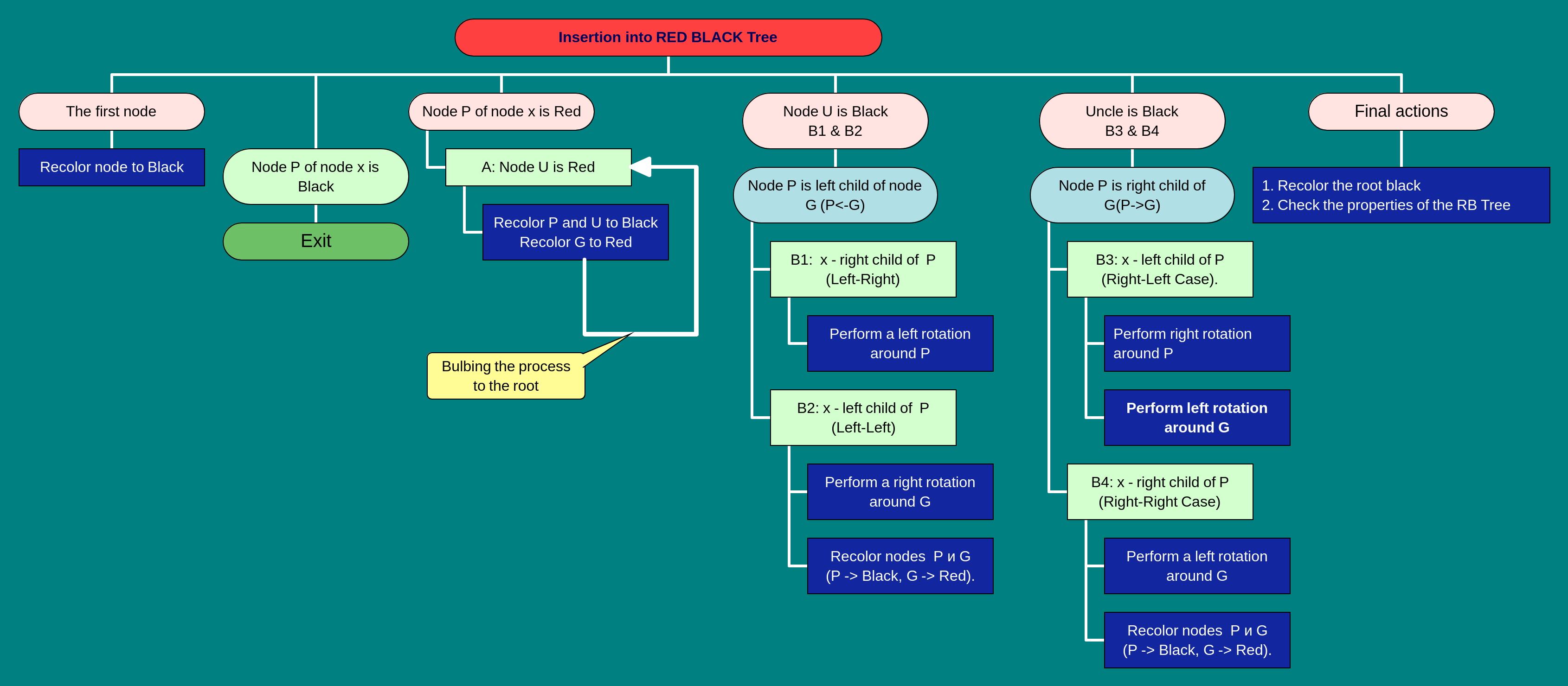
Figure 8.32. Mindmap of the insertion and balancing process

To restore balance, the automaton analyzes the local C-Cluster. Based on the colors and positions of the nodes, it executes the required fix: recoloring (replacing balls) or rotation (rearranging connections). After a local fix, the problem is either resolved or propagates one level up the tree (e.g., a newly colored red ball now sits under a red parent), requiring the automaton to continue its work on the new cluster.

Balancing after insertion is categorized into cases based on the cluster’s configuration. Table 8.1 summarizes these cases, their associated violations, unique signatures, fix criteria, and the mechanical actions applied by the automaton.

Table 8.1. Balancing during insertion in RBT

Case	Violation	Action Type	Cluster Descriptor	Reference Figure
Uncle is Red (Violation State)
Case A	Double Red (U:R)	Recoloring	x:R; P:R; G:B; U:R	Fig8_33a_A_Violation.svg
Uncle is Black (Violation State)
Case B1	Double Red (U:B)	Zig-Zig (LL)	x:R, x<P; P:R, P<G; G:B; U:B, U>G	Fig8_33b_B1_LL_Violation.svg
Case B2	Double Red (U:B)	Zig-Zig (RR)	x:R, x>P; P:R, P>G; G:B; U:B, U<G	Fig8_33c_B2_RR_Violation.svg
Case B3	Double Red (U:B)	Zig-Zag (LR)	x:R, x>P; P:R, P<G; G:B; U:B, U>G	Fig8_33d_B3_LR_Violation.svg
Case B4	Double Red (U:B)	Zig-Zag (RL)	x:R, x<P; P:R, P>G; G:B; U:B, U<G	Fig8_33e_B4_RL_Violation.svg

Case

Violation

Action Type

Cluster Descriptor

Reference Figure

Uncle is Red (Violation State)

Case A

Double Red (U:R)

Recoloring

x:R; P:R; G:B; U:R

Fig8_33a_A_Violation.svg

Uncle is Black (Violation State)

Case B1

Double Red (U:B)

Zig-Zig (LL)

x:R, x<P; P:R, P<G; G:B; U:B, U>G

Fig8_33b_B1_LL_Violation.svg

Case B2

Double Red (U:B)

Zig-Zig (RR)

x:R, x>P; P:R, P>G; G:B; U:B, U<G

Fig8_33c_B2_RR_Violation.svg

Case B3

Double Red (U:B)

Zig-Zag (LR)

x:R, x>P; P:R, P<G; G:B; U:B, U>G

Fig8_33d_B3_LR_Violation.svg

Case B4

Double Red (U:B)

Zig-Zag (RL)

x:R, x<P; P:R, P>G; G:B; U:B, U<G

Fig8_33e_B4_RL_Violation.svg

The visualizations of these distinct violation states — which serve as the 'Atlas' for insertion — are presented in Figures 8.33a-e.

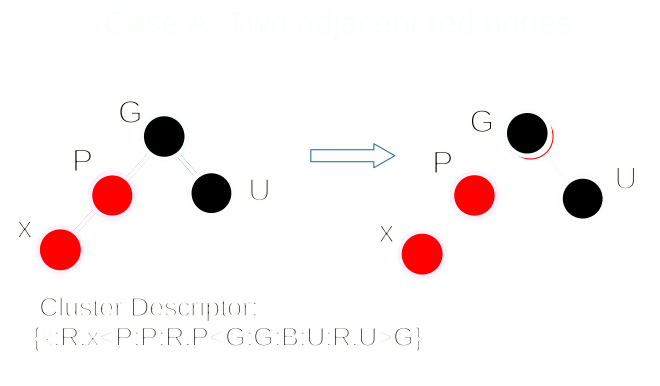
a) Case A — Recoloring (Red Uncle Violation)

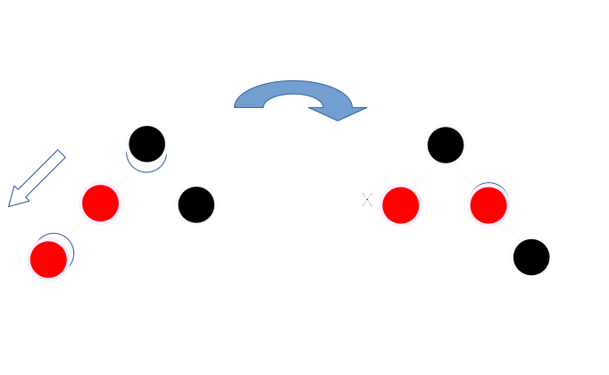
b) Case B1 — Zig-Zig (LL Double Red Violation)

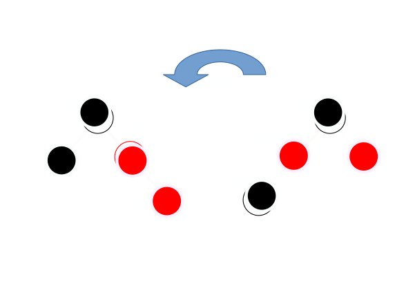
c) Case B2 — Zig-Zig (RR Double Red Violation)

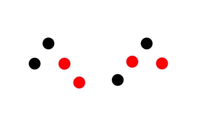
d) Case B3 — Zig-Zag (LR Double Red Violation)

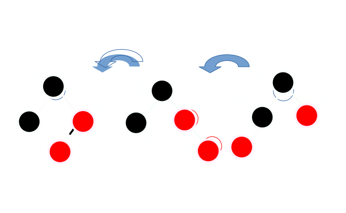
e) Case B4 — Zig-Zag (RL Double Red Violation)

Figure 8.33. Atlas of options (violation states) for balancing after node insertion

The complete logic for red-black tree construction is encapsulated in the rbInsert function (Figure 8.34). It merges standard BST insertion with a call to the specialized fixInsert balancing routine to meticulously restore tree invariants.

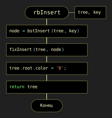
Figure 8.34. DRAKON-diagram of the function rbInsert(tree, data)

The complete decision logic of the balancing process is mapped out in the master DRAKON-diagram shown in Figure 8.35.

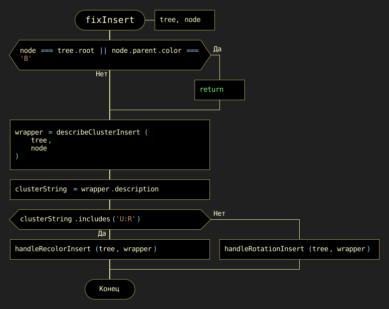
Figure 8.35. DRAKON-diagram of the tree balancing function fixInsert(tree, data)

The internal logic for the recoloring handler (Case A, Red Uncle) is shown in Figure 8.36, while the logic for the rotation handlers (Cases B1-B4, Black Uncle) is detailed in Figure 8.37.

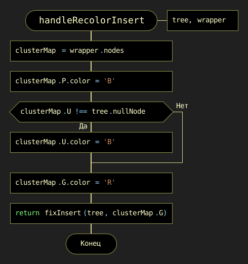
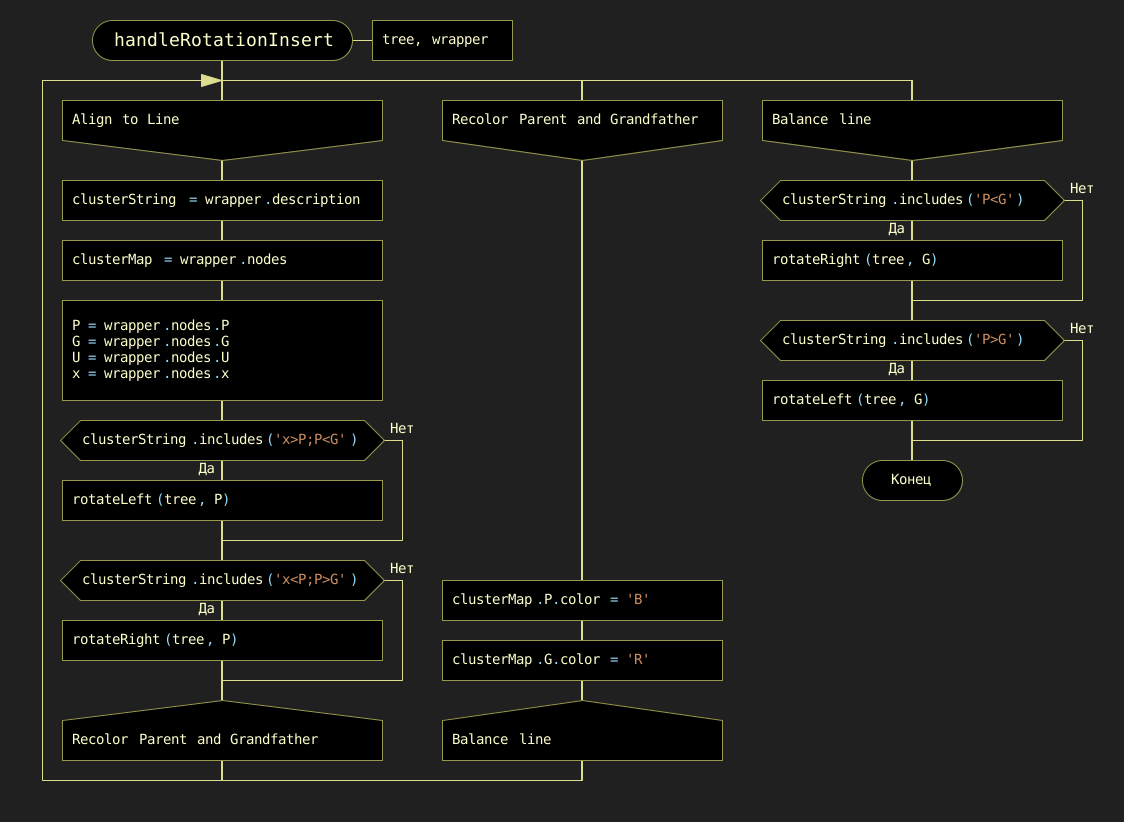
Figure 8.36. DRAKON-diagram of the recoloring algorithm for a red uncle

Figure 8.37. DRAKON-diagram of the rotation algorithms for a black uncle

The fundamental rotation primitives used by these handlers — the "building blocks" of restructuring — are detailed in Figures 8.38a and 8.38b.

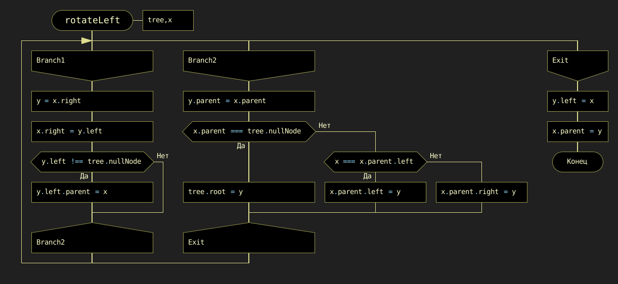
a) Left-rotation primitive

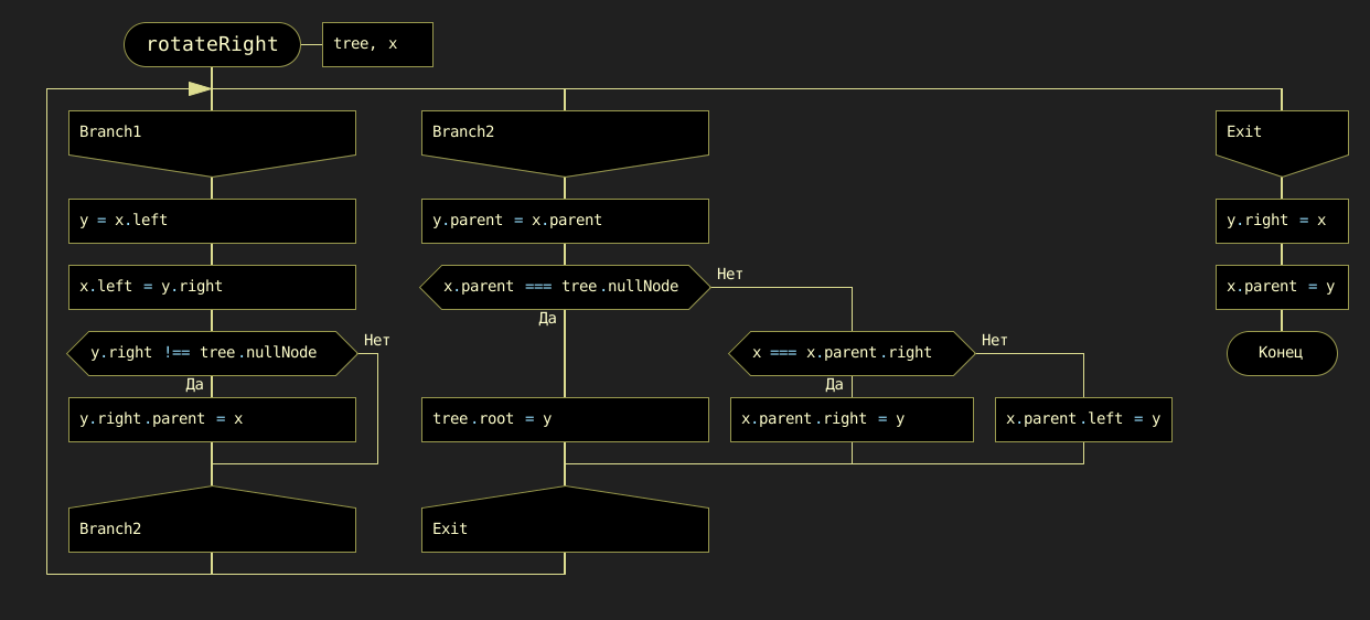
b) Right-rotation primitive

Figure 8.38. DRAKON-diagrams of the fundamental rotation primitives

Deepen your understanding: experiment with the dedicated online visualization and simulation tool, Red-Black Tree Visualizer. This interactive platform allows you to insert and delete nodes, observe the balancing operations in real time, and visualize the tree structure dynamically. Engaging with this tool will enhance your comprehension of the balancing mechanisms described above.

8.4.3. Deleting a Node: Restoring the Weight Balance

Node deletion in a red-black tree is a sophisticated operation because it must preserve the tree’s "gravitational" balance. However, by adhering to our analogy of weights (black nodes) and zero-gravity spacers (red nodes), the logic becomes intuitive: complexity only arises when we lose a "weight."

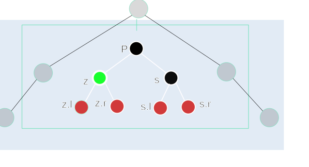
The standard mechanical notation for the C-Cluster used in deletion operations is shown in Figure 8.39:

z: The node to be physically deleted, which triggers the Weight Debt (the "Double-Black" focus).
P: Parent of z.
s: Sibling of z.
s.l, s.r: The left and right children of sibling s (the "nephews").

Figure 8.39. Cluster deletion nodes and their designations (z, P, s, s.l, s.r)

The complete deletion and rebalancing process is summarized in the mindmap in Figure 8.40.

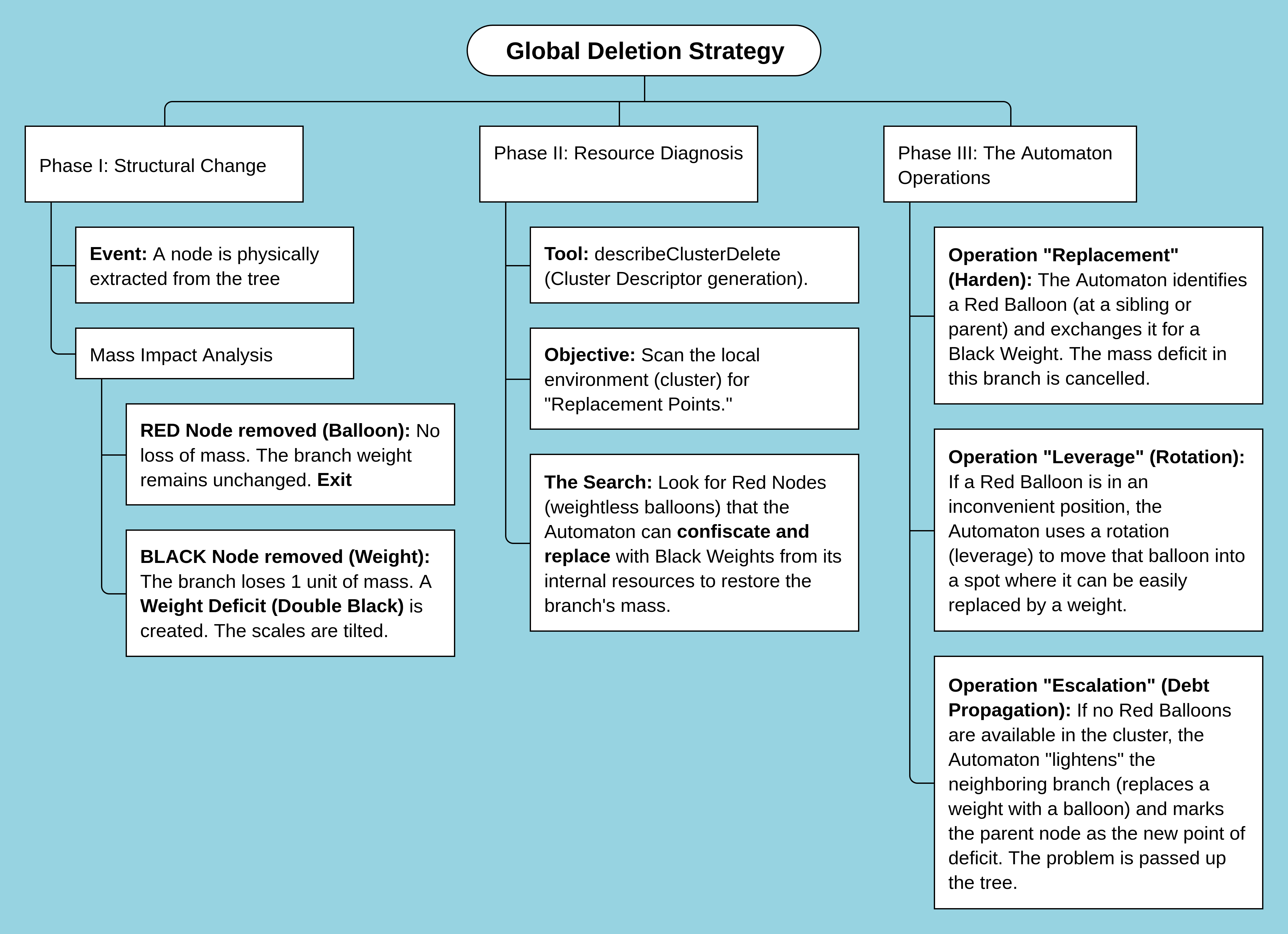
Figure 8.40. Mindmap summarizing RB tree deletion operations

The operation consists of three primary steps:

Identification: As in any standard BST, the algorithm first locates the target node (z).
Structural Deletion and Replacement: We must physically remove the node in a way that minimizes damage:
- If node z has at most one child: we remove z and replace it with its non-NIL child (or a NIL node).
- If node z has two children: we cannot delete it directly. Instead, we find its inorder successor (the minimum node in its right subtree), swap their values, and then delete the successor. This ensures that the node being physically removed always has zero or one child.
The Color Impact (The Weight Factor): Rebalancing necessity is determined entirely by the color of the physically deleted component:
- Deleting a Red Node: if the deleted node is red, no action is required. As red nodes are weightless, their removal does not alter any black-height paths, and Property 5 remains intact.
- Deleting a Black Node: if the deleted node is black, we have a problem. We have removed a "brick" from one side of the scale. This branch is now "lighter," violating Property 5 and creating a Weight Deficit.

This deficit is the core of the "Double Black" problem. It signals to our balancing automaton that it must either:

Find a spare red node in the vicinity and 'harden' it into a weight.
Or redistribute weights from neighboring branches to fill the gap.

The "Double Black" Concept (The Weight Debt): The node that occupies the position of the physically deleted black node is temporarily designated as "Double Black" (DB). In our chandelier analogy, this is a Weight Debt — a conceptual void indicating the path through this node is "lighter" than Property 5 requires. Correcting this violation employs a sequence of recoloring and rotations:

Weight Transfer: Shifting a black weight from a neighboring branch via rotation.
Color Hardening: Transforming a red node into a black weight to fill the void.
Debt Propagation: If the local cluster cannot cancel the void, the "debt" is moved up toward the parent. The parent then becomes the new focus of the balancing process until the deficit is cancelled at the root or resolved by a rotation.

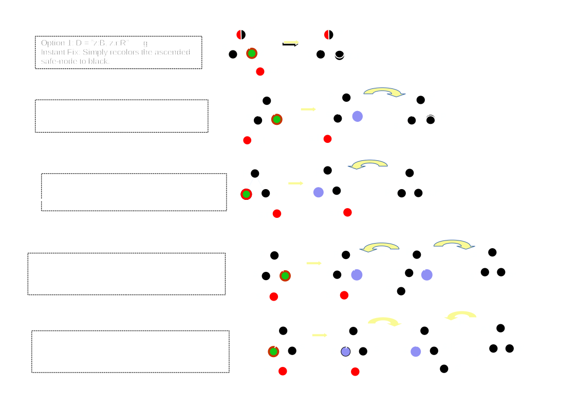
The atlas of options for removing a node from the RB tree is presented in Figure 8.41.

Figure 8.41. Atlas of options for node deletion from the RB tree

The DRAKON-diagram of the deleteNode function, which implements this complex structural logic, is shown in Figure 8.42.

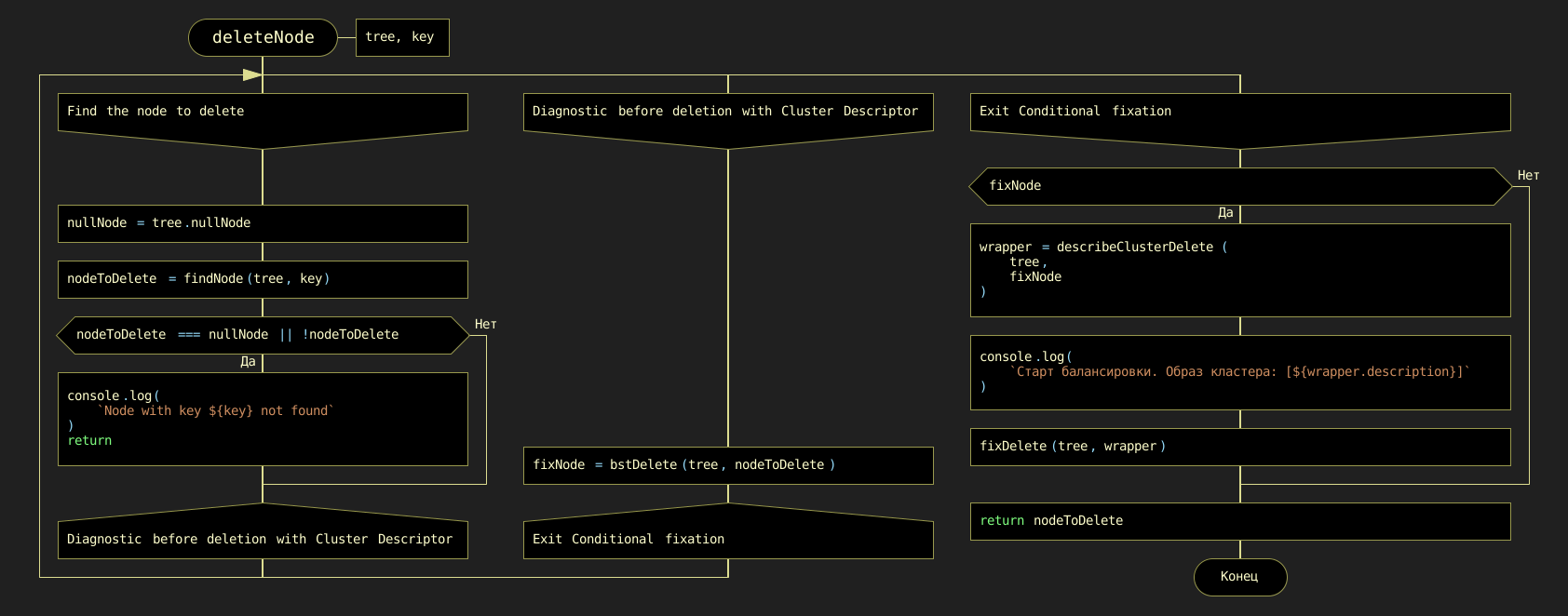
Figure 8.42. DRAKON-diagram of the function deleteNode(tree, data)

To streamline rebalancing, a separate utility function analyzes the cluster state. The DRAKON-diagram for deleteClusterDescriptor, which generates the unique 'signature' string, is shown in Figure 8.43.

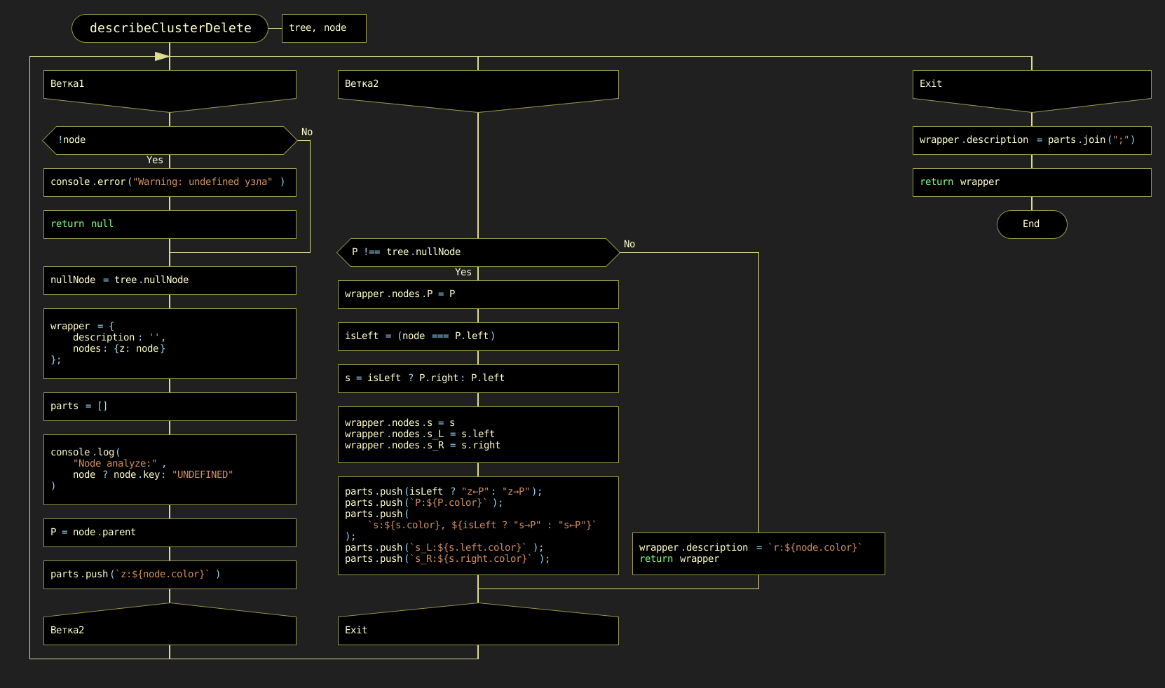
Figure 8.43. DRAKON-diagram of the descriptor function deleteClusterDescriptor(tree, data)

Once the cluster is analyzed, the balancing automaton function fixDelete(tree, data) acts upon the result. It makes all high-level balancing decisions based on the descriptor signature. Its DRAKON-diagram is presented in Figure 8.44.

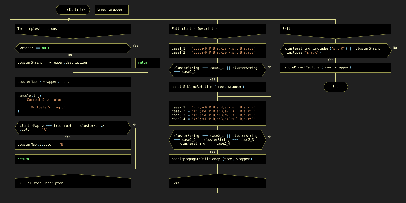
Figure 8.44. DRAKON-diagram of the automaton dispatcher function fixDelete(tree, data)

As detailed in the mapping table below, the dispatcher fixDelete distributes tasks among three specialized "handlers." The names of these functions (handleSiblingRotation, propagateDeficiency, handleDirectCapture) precisely reflect the specific action of the control automaton.

Table 8.2. Mapping automaton purpose to specialized function names (handle types)

Automaton Purpose in the Atlas	Proposed Function Name (handle type)
Maneuver with a Red Sibling (s:R) Goal: Make sibling s black so the automaton can capture a resource in the next step. The deficiency is not resolved.	handleSiblingRotation
Deficiency Propagation (s:B, no resources) Goal: "Dissolve" the deficiency (z) by recoloring sibling s to red, and move the deficiency (blue tag) to parent P.	propagateDeficiency
Final Black Height Recovery (s.l:R or s.r:R) Goal: Find and capture a red resource (s.l or s.r) by performing rotations and recoloring. The deficiency is completely resolved (Options 2a-2d).	handleDirectCapture

Automaton Purpose in the Atlas

Proposed Function Name (handle type)

Maneuver with a Red Sibling (s:R)
Goal: Make sibling s black so the automaton can capture a resource in the next step. The deficiency is not resolved.

handleSiblingRotation

Deficiency Propagation (s:B, no resources)
Goal: "Dissolve" the deficiency (z) by recoloring sibling s to red, and move the deficiency (blue tag) to parent P.

propagateDeficiency

Final Black Height Recovery (s.l:R or s.r:R)
Goal: Find and capture a red resource (s.l or s.r) by performing rotations and recoloring. The deficiency is completely resolved (Options 2a-2d).

handleDirectCapture

The complete DRAKON-diagrams detailing the internal logic of these three specialized functions are shown in Figures 8.45a, 8.45b, and 8.45c.

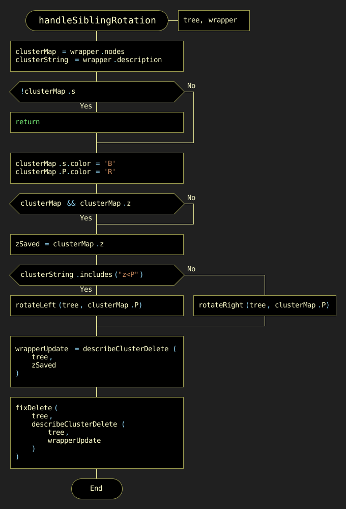
a) handleSiblingRotation

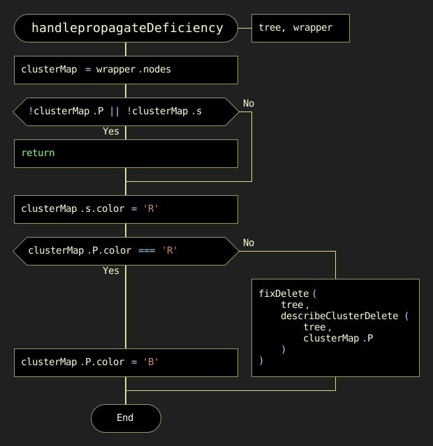
b) propagateDeficiency

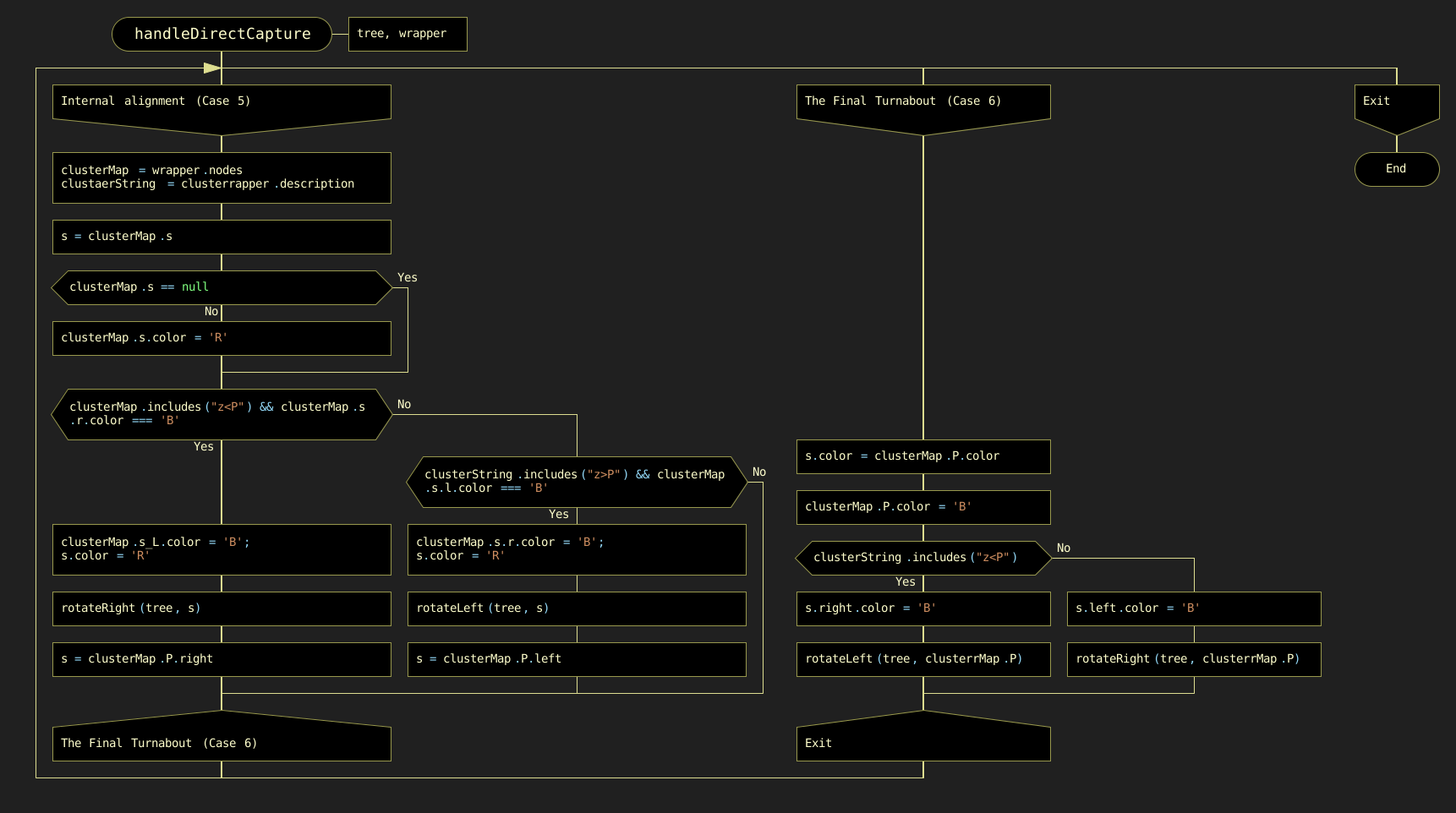
c) handleDirectCapture

Figure 8.45. DRAKON-diagrams of the three specialized handle-type functions for RB tree balancing

8.5. Comparison of Tree Structures

A clear comparison of the dynamic behavior of each tree structure is presented in Table 8.3. While standard BST implementations risk degrading into linear structures with O(n) complexity, self-balancing structures (AVL and red-black) guarantee O(log n) complexity, making them scalable for large datasets. Note that although red-black trees have dynamic complexities in insertions and deletions compared to BSTs, they eliminate the critical O(n) failure mode, providing a predictable O(log n) experience.

Table 8.3. Comparison of time and space complexities for tree operations

Tree Type	Operation	Average Time Complexity	Worst-Case Time Complexity	Space Complexity
BST	Insert	O(log n)	O(n)	O(n)
Find	O(log n)	O(n)	O(n)
Delete	O(log n)	O(n)	O(n)
AVL Tree	Insert	O(log n)	O(log n)	O(n)
Find	O(log n)	O(log n)	O(n)
Delete	O(log n)	O(log n)	O(n)
Red-Black Tree	Insert	O(log n)	O(log n)	O(n)
Find	O(log n)	O(log n)	O(n)
Delete	O(log n)	O(log n)	O(n)

Tree Type

Operation

Average Time Complexity

Worst-Case Time Complexity

Space Complexity

BST

Insert

O(log n)

O(n)

Find

O(log n)

O(n)

Delete

O(log n)

O(n)

AVL Tree

Insert

O(log n)

O(n)

Find

O(log n)

O(n)

Delete

O(log n)

O(n)

Red-Black Tree

Insert

O(log n)

O(n)

Find

O(log n)

O(n)

Delete

O(log n)

O(n)

Computational Experiment

More information about the experiment can be found in the App by activating the "Launch Sorting Experiment" button.

Run experiment

8.6. Conclusion

Trees are one of the most important data structures in computer science, used to represent hierarchical relationships and organize data. They provide efficient search, insert, and delete operations, making them ideal for use in a variety of applications.

AVL trees, named after their creators Adelson-Velsky and Landis, are balanced binary search trees. They provide fast search, insertion, and deletion by keeping the height of the tree logarithmic relative to the number of nodes. However, AVL trees require additional insertion and deletion operations to maintain balance, which can be a disadvantage in some applications.

Red-black trees are another type of balanced binary search tree. They provide efficient search, insert, and delete operations, but can be more difficult to implement because of the additional properties they must support. They are widely used in many standard libraries.

The choice of a specific tree type depends on the specific requirements of the application. AVL trees are generally preferred when frequent searches are the most important operations, as they provide a more stringent balance than red-black trees. On the other hand, red-black trees can be more effective with frequent insertions and removals, as they require fewer rotations to maintain balance.

It is important to remember that both types of trees require additional memory to store balance information, and both can be difficult to implement. In some cases, other data structures, such as hash tables or B-trees, may be more appropriate. However, despite these challenges, trees continue to play a central role in computer science and are a key tool for any programmer.