Section 10. Data Structures Selection in Practice

10.1. Data Structure Selection Roadmap

Choosing an optimal data structure is a multi-criteria decision problem that requires consideration of functional requirements, data characteristics, the operation profile, and physical hardware constraints. Functional requirements answer the question “What operations must be supported?”, the operation profile answers “How often and under what conditions will these operations be performed?”, and hardware constraints answer “What resources are available, and how do they affect performance?”

Functional requirements specify which operations on data a structure must support and which properties it must preserve. Examples include lookup by key, insertion and deletion of elements, access by index, maintaining sorted order, and retrieving values within a specified range. These requirements establish the set of suitable data structures.

The operation profile describes how a structure will be used: which operations are performed most frequently, the volume of data they involve, and their sequence. For example, one application may primarily perform lookups, with infrequent updates; another may continuously receive new elements and then process them sequentially. Even when the required operations are identical, differences in their execution frequency may lead to the selection of different structures.

The hardware constraints of the system impose additional limitations on the choice of data structures. These constraints include the available RAM capacity, cache size and line size, memory access latency, memory bandwidth, pointer size and alignment requirements, parallel processing capabilities, and storage device characteristics. Each of these factors can significantly impact the performance of different data structures (Table 1).

Table 1. Hardware Characteristics and Constraints

Factor	Impact on data structure selection
Available RAM capacity	In addition to the data itself, a structure stores auxiliary information: pointers, indices, and reserved slots. This overhead may limit the maximum size of the structure.
Cache capacity and cache line size	Storing elements close together allows several adjacent values to be loaded in a single memory access and subsequently used without accessing RAM again.
Memory access latency	Particularly significant when following a chain of pointers: the address of the next element becomes available only after the previous element has been read.
Memory bandwidth	Limits the speed of bulk scanning, copying, and moving data, for example when inserting elements into an array.
Pointer size and alignment requirements	Affect the actual memory footprint of elements: pointers and alignment padding can substantially increase memory usage.
Parallel processing capabilities	When multiple cores are used, data partitioning and the frequency of access to shared memory become important. Contention over the same cache lines can reduce performance.
Storage device characteristics	When data does not fit in RAM, the number of storage accesses and the size of transferred blocks become important. This is one reason for using B-trees and B+ trees.

Factor

Impact on data structure selection

Available RAM capacity

In addition to the data itself, a structure stores auxiliary information: pointers, indices, and reserved slots. This overhead may limit the maximum size of the structure.

Cache capacity and cache line size

Storing elements close together allows several adjacent values to be loaded in a single memory access and subsequently used without accessing RAM again.

Memory access latency

Particularly significant when following a chain of pointers: the address of the next element becomes available only after the previous element has been read.

Memory bandwidth

Limits the speed of bulk scanning, copying, and moving data, for example when inserting elements into an array.

Pointer size and alignment requirements

Affect the actual memory footprint of elements: pointers and alignment padding can substantially increase memory usage.

Parallel processing capabilities

When multiple cores are used, data partitioning and the frequency of access to shared memory become important. Contention over the same cache lines can reduce performance.

Storage device characteristics

When data does not fit in RAM, the number of storage accesses and the size of transferred blocks become important. This is one reason for using B-trees and B+ trees.

Before making a choice,you must define the mandatory operations (key-based lookup, indexed access, insertion, deletion, range queries) and the required data organization properties (key ordering, insertion-order preservation, element uniqueness, or allowing duplicates). Data structures that fail to meet these requirements are ruled out from further consideration.

Data structure selection algorithm according to the characteristics of a specific task can be presented in five steps (Figure 10.1. )

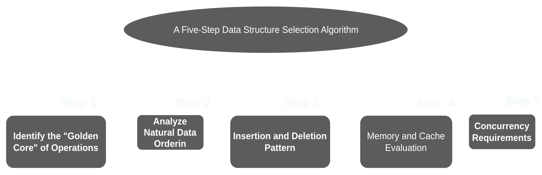
Figure 10.1. Multi-Criteria Memory-Oriented decision-making algorithm for data structure selection

In more detail Multi-Criteria Memory-Oriented decision-making algorithm for data structure selection is presented in the following tables (Tables 2.1–2.5).

Table 2.1. Step 1: Identifying the Operation Profile (“Golden Core”)
Criterion / Condition	Candidate Data Structures	Engineering Rationale and Considerations
Mostly reading and searching	Arrays for indexed access or sequential traversal; hash tables for lookup by key; sorted arrays or balanced search trees for ordered queries.	Distinguish direct access, lookup by key, and sequential traversal. These operations have different costs and may favor different structures.
Mostly writing and insertion	Dynamic arrays for appending; linked lists for insertion at known locations; hash tables or balanced search trees for updates by key.	The insertion location and subsequent access requirements determine which candidates are appropriate. For LIFO or FIFO processing, choose a suitable stack or queue implementation.
Mixed read/write workload	Dynamic arrays, hash tables, or balanced search trees, depending on the required operations.	Compare the frequency and cost of each operation. Reserving capacity, where supported, can reduce reallocations or rehashing but consumes additional memory.

Operation frequencies alone do not determine the best structure: data volume, insertion locations, and the cost of each operation also matter. Ratios such as 80/20 or 50/50 illustrate workloads; they are not universal selection thresholds. Stacks and queues specify access disciplines and can be implemented using different underlying structures.

Table 2.2. Step 2: Assessing the Need for Data Ordering
Criterion / Condition	Candidate Data Structures	Engineering Rationale and Considerations
Key order is required (range queries, ordered traversal, predecessors and successors)	Balanced search trees (AVL or red-black trees), B-trees or B+ trees, skip lists, and sorted arrays.	These structures support operations based on key order. The update frequency and storage environment help distinguish between them; a hash table alone does not provide ordered range queries.
Key order is not required (individual lookups by key)	Hash table.	Expected O(1) lookup is possible under suitable hashing and load-factor assumptions, assuming bounded-cost key hashing and comparison. Worst-case lookup is not generally O(1).

Key order and insertion order are different requirements: preserving insertion order does not make keys sorted. If only the minimum or maximum must be retrieved repeatedly, a heap may suffice; maintaining full key order may be unnecessary.

Table 2.3. Step 3: Identifying the Insertion and Deletion Pattern
Criterion / Condition	Candidate Data Structures	Engineering Rationale and Considerations
Insertion and deletion at the end only	Dynamic array; a stack implemented using a dynamic array or linked nodes.	Dynamic-array append is amortized O(1); removing the last element does not require shifting the remaining elements. Occasional resizing may move existing elements.
Insertion and deletion at the beginning only	Linked list with a head reference; deque with efficient operations at the front.	These implementations avoid the O(n) element shifting required by a conventional contiguous array when its front changes.
Insertion at one end and removal at the other, or changes at both ends	Queue or deque implemented using a circular buffer or an appropriately linked structure.	A circular buffer reuses vacant positions without shifting all elements. A linked implementation requires suitable head and tail references; efficient removal at both ends generally requires backward links.
Insertion or deletion at an internal position	Dynamic array for infrequent changes; linked list when the required node references are already available.	Array changes may shift O(n) elements. A list can change links in O(1), but locating the position may require an O(n) traversal; frequent insertion alone does not establish that a list is preferable.
Insertion, update, or deletion by key	Hash table when key order is unnecessary; balanced search tree when ordered operations are required.	Hash tables typically provide expected O(1) key-based operations under suitable assumptions; balanced search trees provide O(log n) search, insertion, and deletion under the usual comparison-cost model.

The total cost includes locating the target and modifying the structure. Constant-time link changes require access to all necessary nodes; for example, deleting a node from a singly linked list generally requires its predecessor. Changing an element by key and inserting at a numerical position are different tasks.

Table 2.4. Step 4: Assessing Memory and Cache Constraints (Hardware Filter)
Criterion / Condition	Candidate Data Structures	Engineering Rationale and Considerations
Small working set with frequent sequential access	Contiguous arrays or other compact representations.	Good spatial locality can reduce memory-access overhead. Element shifting may be acceptable for small arrays, but its actual cost depends on element size, workload, and hardware.
Large data volume in RAM with frequent sequential processing	Arrays or chunked arrays.	Compact or block-based storage supports efficient scanning and reduces per-element pointer overhead. A large data volume alone does not justify choosing a linked list.
Large data volume in RAM with frequent localized changes	Balanced search trees for changes by key; linked lists when the necessary node references are known; chunked structures when suitable.	These candidates can avoid shifting a large contiguous suffix, but pointer overhead, allocation costs, and cache misses must be weighed against that benefit.
Data exceeds available RAM or is primarily stored on a storage device	B-trees or B+ trees for indexed access and updates; block-oriented sequential layouts for scans.	Match the layout to the access pattern. Block-oriented trees reduce the number of storage accesses for indexed operations, while sequential layouts favor bulk processing.
Read-only data requiring lookup or traversal in key order	Sorted array with binary search.	A compact representation supports O(log n) binary search and efficient sequential traversal. Binary search has a different access pattern from a sequential scan and does not obtain the same predictable streaming-prefetch benefit.

Performance depends on the active working set, element layout, access pattern, and implementation; no universal cache-size or timing threshold determines the winner. In JavaScript, an ordinary Array does not guarantee the same physical representation as a packed numeric buffer; TypedArray provides a clearer model for fixed-width numeric data. Validate candidate implementations using representative data and workloads.

Table 2.5. Step 5: Determining Whether Concurrent Access Is Required
Criterion / Condition	Candidate Data Structures / Access Strategies	Engineering Rationale and Considerations
Several threads or workers process independently owned data	Separate structures per thread or worker; partitioned data with explicit ownership and communication.	Independent ownership can reduce contention. Exchanging data or combining results may still require coordination.
Several threads or workers access shared mutable data	Structures protected by locks; partitioned structures with appropriate coordination; specialized concurrent structures, including lock-free queues where justified.	Choose according to the required consistency guarantees, contention level, and runtime support. Lock-free algorithms are one option, not an automatic consequence of using multiple threads.
Single-threaded execution without concurrent shared-memory access	Simple implementations appropriate to the required operations.	No inter-thread synchronization is needed, reducing coordination overhead and implementation complexity.

First identify which data is shared, which operations modify it, and which guarantees must hold during concurrent access. Lock-free does not mean synchronization-free or necessarily faster; such algorithms require suitable atomic operations and careful implementation. In JavaScript, asynchronous execution alone does not imply parallel shared-memory access.

Conclusion

The five-step algorithm presented here makes it possible to identify data structures that meet the requirements of the task at hand. Functional requirements define the set of viable solutions, while the operation profile, the nature of data mutations, and the constraints of the computing environment help compare the remaining candidates. The result is a well-grounded choice of one or more candidates, which must then be validated on representative data and workloads by measuring operation execution time and memory consumption.

Applying the hardware filter introduced in the fourth step requires understanding how the elements of a structure are placed in computer memory and how the processor accesses them. Sequentially reading adjacent array elements versus following references between list nodes can incur substantially different time costs, even when processing the same number of elements.

The next subsection therefore examines the memory hierarchy and its impact on data structure performance. This will help explain why the theoretical advantages of a structure do not always translate into faster performance in a real computing environment.

10.2. Memory Hierarchy and Its Impact on Data Structure Performance

Any practical choice of a data structure in a real computing system must account not only for the abstract algorithmic complexity (Big-O) but also for the physical organization of memory. Ignoring this factor is one of the primary reasons why a theoretically optimal structure often performs slower in practice than a "simpler" alternative.

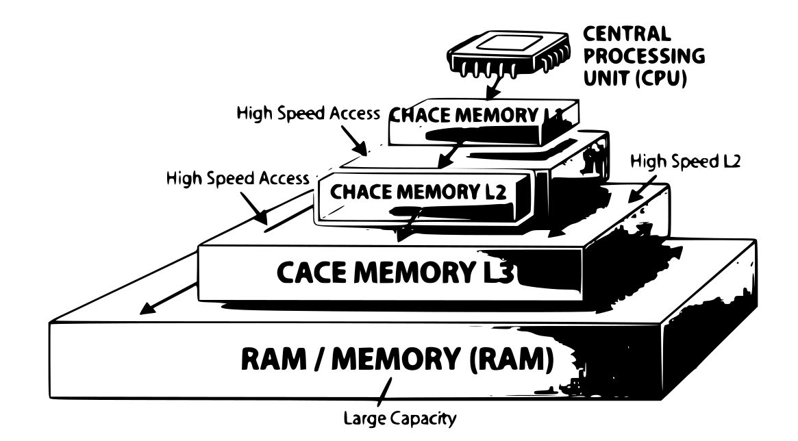
In modern computers, memory is organized as a hierarchical pyramid (Figure 10.2), where each level differs in capacity, access speed, and cost.

Figure 10.2. Memory hierarchy of a modern computer

10.2.1. Characteristics of Memory Levels

Each memory level has unique parameters that determine how efficiently a particular data structure interacts with it. The figures below are order-of-magnitude estimates for a typical modern system, not measurements of any specific processor — actual numbers vary with microarchitecture, process node, and generation of hardware. Bandwidth values are especially approximate: they depend on the number of cores and memory channels.

Memory level comparison
Memory Level	Typical Size	Access Time	Bandwidth	Managed By	Relative Energy
CPU Registers	~1 KB	< 1 ns	~100 GB/s	Compiler	1×
L1 Cache	32–64 KB	~1 ns	~50 GB/s	Hardware	2×
L2 Cache	256–512 KB	~3–5 ns	~30 GB/s	Hardware	4×
L3 Cache	4–32 MB	~10–15 ns	~20 GB/s	Hardware	8×
RAM	8–256 GB	~50–100 ns	~10–20 GB/s	OS/Program	20×
SSD/Disk (swap)	256 GB – 4 TB	~50–200 μs (SSD) / ~10 ms (HDD)	~0.5–5 GB/s	OS	1000×

Important: The difference between register access time (< 1 ns) and RAM access time (~100 ns) is two orders of magnitude. In the time the CPU waits for data from RAM, it could have executed hundreds of operations. This is precisely why data structures that are "cache-friendly" can outperform even those with better theoretical complexity.

10.2.2. Key Concepts: Cache Line and Cache Miss

The CPU does not work with individual bytes but with fixed-size blocks called cache lines (typically 64 bytes). When a program accesses a variable, the entire cache line containing that variable is loaded into the cache.

Cache hit: Data is already in the cache. Access takes ~1 ns (L1) and a few nanoseconds for L2.
Cache miss: Data is not in the nearest cache level and must be fetched from a slower one. If it is not in any cache, it is loaded from RAM; latency is ~100 ns (up to 100× slower than an L1 hit).

For data structures, this means:

Arrays (and any sequentially stored structures): When iterating over an array, the CPU loads one cache line (64 bytes = 8 elements of 8 bytes) and processes all 8 elements without additional misses. This achieves near-theoretical maximum speed.
Linked lists and trees: If nodes are scattered across memory, moving to the next node almost always causes a cache miss, because the adjacent node does not reside in the same cache line. The latency accumulates, and iteration can become 5–20 times slower than over an array.

In JavaScript, an ordinary Array does not guarantee a contiguous block of fixed-width numbers. When the cache-friendly layout matters, use a TypedArray (for example, Float64Array or Int32Array), which stores numbers in one contiguous buffer.

10.2.3. Prefetching Mechanism

Modern processors feature hardware prefetchers that analyze memory access patterns and proactively load data into the cache.

For arrays, the prefetcher works very well: it detects linear traversal and begins loading cache lines ahead, before the program even requests them. This largely hides RAM latency.
For linked lists and trees, the prefetcher can rarely help: the address of the next node becomes known only after the current node has been read, so the CPU cannot anticipate where the program will jump next. The exception is a list or tree whose nodes happen to lie close together in memory (for example, nodes created one after another in an otherwise empty heap); then the access pattern is regular and the penalty is much smaller.

Conclusion: A full traversal of any of these structures takes O(n) steps, but the cost of a step differs. If your data structure is traversed frequently, an array step is typically several times to an order of magnitude cheaper than a step over scattered list or tree nodes. Complexity classes alone do not show this difference.

10.2.4. Practical Rule: The "Cache Filter"

When selecting a data structure, always ask yourself three questions:

Will the structure be iterated (traversed entirely) frequently?
- YES → Prefer arrays and vectors, unless the structure is modified far more often than it is traversed (an O(n) insertion may then cost more than the savings).
- NO → Trees and lists become viable options.
What is the access pattern?
- Sequential (in order) → Arrays win due to prefetching.
- Random (by index or key) → Hash tables and trees provide the advantage.
How large is the data in bytes, compared with the cache sizes? Estimate the size as the number of elements multiplied by the size of one element, including pointers and per-node overhead. For example, one million 8-byte numbers occupy 8 MB in an array, while the same numbers in linked-list nodes with a pointer and allocator overhead can occupy two to four times as much.
- Data fits in L3 (a few MB up to tens of MB) → A cache miss is served from L3 in ~10–15 ns, so the penalty of following pointers is moderate.
- Data does not fit in L3 → Every pointer jump may go to RAM (~50–100 ns). An array still streams efficiently thanks to prefetching, so the gap between arrays and pointer-based structures is typically at its largest here.

10.2.5. Illustrative Example: Iterating 1 Million Elements

Consider three data structures, each containing 1 million integers. We perform a full iteration and measure time. The numbers below are illustrative estimates for a typical modern desktop processor and an unfavorable case in which the list and tree nodes are scattered in memory; measure on your own hardware before drawing conclusions.

Iteration performance comparison
Structure	Memory Layout	Cache Misses per Element	Relative Time	Estimated Real Time
Array	Sequential	~0.125 (1 miss per 8 elements)	1×	~1 ms
Linked List	Scattered	~1 (almost always a miss)	~15×	~15 ms
Tree (depth-first traversal)	Scattered	~1–1.5	~20×	~20 ms

Important: This timing is only for full iteration. If the structure is used for search (not iteration), the picture changes: a hash table gives expected O(1) lookup, a balanced tree or a sorted array gives O(log n), and an unsorted array requires O(n). Iterating over an open-addressing hash table scans one array that includes empty slots, so it is typically slower than a dense array but much closer to it than to a list or a tree. Therefore, the choice always depends on the dominant operation.

To reproduce the effect in your own experiment, the nodes must really be scattered. Nodes created one after another often occupy neighboring addresses, and such a list behaves much closer to an array. Build the list, then shuffle the order of its nodes (or interleave the allocations with other data) before measuring.

10.2.6. Cache-Friendly Structures (Priority During Selection)

Based on memory hierarchy analysis, we can construct a qualitative cache-locality rating for major data structures:

Cache-locality rating
Friendliness Level	Data Structures	Reason
Excellent (★★★★★)	Static Array, Dynamic Array (Vector), Sorted Array	Sequential storage, effective prefetching
Good (★★★☆☆)	Hash Table (open addressing), Deque (array-based)	Elements are scattered but within a single allocation
Fair (★★☆☆☆)	Linked List (with node pool), Red-Black Tree (with custom allocator)	Nodes are scattered, but a pool improves locality
Poor (★☆☆☆☆)	Naive Linked List, AVL/RBT with standard new/malloc	Each node is a separate allocation, maximal fragmentation

10.2.7. Bridge to the DRAKON Decision Diagram

Understanding the memory hierarchy explains the hardware filter of the data structure selection algorithm (Step 4 in Section 10.1, Figure 10.1):

If cache locality is a priority (high-load systems, game engines, financial applications) → favor arrays and sequentially stored structures.
If cache locality is not critical (background tasks, batch processing, infrequent access) → trees and lists can be chosen without concern.

This filter is applied after the questions about the operation profile and ordering and before the question about concurrent access, as shown in Figure 10.1.

Based on the material in this subsection, the following procedure can be proposed for assessing the resources available for a specific task.

Procedure for Assessing Available Resources for a Specific Task
What to Assess	What Needs to Be Determined	How It Affects the Decision
Data volume and expected growth	Number of elements, size of a single element, possible maximum volume	Helps assess whether the data will fit in available memory
Total memory consumption	Beyond the useful data itself: references, indices, reserved capacity, temporary copies, and auxiliary structures	Compact source data does not necessarily mean low memory consumption for the program as a whole
Available RAM	How much memory can be allocated to the program, accounting for the OS, runtime environment, and other processes	A margin should be left for data growth and peak consumption during operations
Working set and locality	Which portion of the data is actively used; whether accesses are sequential or reference-based	Helps assess the benefit of compact placement and the likelihood of data reuse from cache
Nature of memory and storage exchange	Whether bulk reads/copies predominate, or numerous scattered accesses	In the first case, throughput matters most; in the second, the latency of individual accesses
Parallel processing capability	Whether data and work can be split across executors; which data will remain shared	Indicates whether additional cores can be leveraged without excessive coordination overhead
Actual program metrics	Time for characteristic operations, peak memory consumption, behavior under increasing load	Allows preliminary estimates to be verified and implementations compared in the target environment