Section 5. Complexity and Stability Analysis of Algorithms
This section introduces the analysis of algorithm complexity and stability as essential tools for evaluating algorithm quality. It explains that a correct algorithm must not only produce the expected result, but also terminate in a finite number of steps and use time and memory resources efficiently. The section presents theoretical complexity analysis through an abstract machine model, allowing algorithms to be compared independently of a specific computer or JavaScript runtime. Special attention is given to asymptotic notation, including Big-O, Omega, and Theta, and to common complexity classes such as constant, logarithmic, linear, and quadratic complexity. JavaScript examples are used to connect these mathematical ideas with practical code behavior, while DRAKON diagrams can help visualize control flow and repeated operations that influence complexity. The section also introduces space complexity and algorithm stability, preparing the reader to evaluate algorithms by correctness, performance, memory usage, and preservation of data order.
5.1. Requirements for Algorithms
The previous sections focused on the description of the most common data structures, on the one hand as abstract entities, and on the other — their concrete implementation in the JavaScript programming language. This section will deal with the theoretical analysis of algorithms for processing data structures from the perspective of estimating the time spent on program code execution and computer memory usage.
In theory and in practice, data structure processing algorithms are defined as a set of sequentially performed, well-defined procedures that provide a final computational result based on a fixed and limited set of source data. Most data processing algorithms include basic data processing procedures such as searching, sorting, adding, updating, deleting, etc.
Foremost, it should be noted that a "good algorithm" must have two characteristics: a) correctness and b) finiteness. Correctness means that if an algorithm is designed to solve a particular problem, it must always produce the correct result for all source data, and no input data will yield the wrong result. The finiteness of an algorithm means that a finite number of computational operations must be performed to obtain the result — that is, the execution of the program code must stop at some point in time.
Once the algorithm is correct and finite, the most important characteristic of the algorithm is efficiency, which is achieved by meeting the following requirements:
-
The algorithm should effectively use the resources available to the system.
-
The computational time (time taken to generate output data corresponding to particular input data) should be minimal.
-
The memory used by the algorithm should also be as small as possible.
In most computational tasks, it is necessary to strive for a compromise between computation time and occupied memory. In other words, when choosing a method for solving a computational problem, you need to decide on priorities: what is more important — computation time or amount of memory occupied. It may seem that this is not so important for modern computers. This becomes critical for large-scale problems — for example, in artificial intelligence or bioinformatics, such as genome decoding. Here, finding the right balance between time and memory is often the deciding factor. In this regard, we will define the term "algorithm complexity" as a measure of the amount of time and/or space required to solve a problem, depending on the size of the data.
Such analysis involves determining a function that links the length of the input data of the algorithm to the time it takes (its time complexity) or the number of storage locations it uses (space complexity). An algorithm is considered effective when the values of this function are either negligible or slowly increasing relative to the size of the input data.
5.2. Theoretical Analysis of Algorithm Complexity
Ultimately, the created algorithms must be implemented on some computing device using the generated program code. Therefore, one should distinguish between the complexity of the algorithm itself and the complexity of its computer implementation. The fastest algorithm implemented on a slow computing device may be less efficient than a less successful algorithm implemented on a computer with more processing power or a programming language capable of parallel computing.
Thus, when assessing the complexity of algorithms, they are evaluated on an abstract machine with random access to memory, which makes it possible to ignore the low-level parameters of the computing device (processor memory size, multitasking, etc.). The model of such a machine consists of memory and a processor, which work as follows:
-
Memory consists of cells, each of which has an address and can store one data element.
-
Each memory call takes one unit of time, regardless of the number of the addressable cell.
-
The amount of memory is sufficient to execute any algorithm.
-
The processor performs any elementary operation in one time step.
-
Loops and functions are not considered elementary operations.
The complexity T(n) of an algorithm associated with estimates of its complexity is determined by counting the number of operations performed. For example, consider the algorithm for finding the maximum element of an array:
const array = [11, 9, 17, 45, 411];
let maxNumber = array[0];

for (let index = 1; index < array.length; index++) {
if (array[index] > maxNumber) {
maxNumber = array[index];
}
}
console.log("The largest value of an array element =", maxNumber);
When implementing this algorithm, the following will be performed:
-
(N - 1) operations of assigning a new value to the loop counter i;
-
(N - 1) operations of comparing the counter with the value N;
-
(N - 1) operations of comparing an array element with the value of maxNumber;
-
(From 1 to N) operations of assigning a value to the variable maxNumber.
It is obvious that such a calculation for determining the complexity of an algorithm and estimating its complexity is individual and depends on the size of the input data. Therefore, it was quite natural to propose a qualitative assessment of complexity depending on the "quality" of the initial data: the best case, the worst case, and the average case.
5.3. Qualitative Assessment of Complexity
Asymptotic notations such as Omega notation (Ω), Theta notation (Θ), and Big-O notation (O) that reflect the three time bounds of an algorithm (lower, middle, and upper) are used to quantify the complexity of algorithms.
-
Omega notation (Ω) represents the lower bound of the algorithm’s running time, which characterizes the best algorithm complexity in terms of achieving efficiency. For any value of n of the source data, the minimum time required by the algorithm is set to Ω(f(n)).
-
Big-O notation (O) represents the upper bound on the execution time of the algorithm, which characterizes the worst complexity of the algorithm in terms of efficiency. In most practical cases, this notation is used to evaluate the effectiveness of algorithms, since it is the worst-case scenario of the computational process that the software developer must evaluate.
-
Theta notation (Θ) represents both an upper and lower bound on the execution time of algorithms and is used to analyze their average complexity.
Consider in more detail the Big-O notation that determines the upper bound of any algorithm — that is, the algorithm cannot take longer than the upper bound.
Constant Time Complexity — O(1)
An algorithm with constant time complexity requires the same amount of time regardless of its input data. For example, given two numbers, you need to calculate their sum.
Logarithmic Time Complexity — O(log n)
When the time taken by an algorithm is proportional to the logarithm of the input size n, it is said to have logarithmic time complexity. An example is the simple calculation of the number of print operations of the index in a loop:
let n = 16;
for (let i = 1; i < n; i *= 2) {
console.log("i = ", i);
}
Recall that log₂ 16 = log₂ 2⁴ = 4 log₂ 2 = 4, since log₂ 2 = 1. Algorithms with logarithmic complexity are considered highly efficient because the ratio of execution time to the size of the data array decreases as the data size increases. Algorithms that work in logarithmic time are usually found in binary tree operations or binary search operations. Such algorithms will be discussed in the next section.
Linear Time Complexity — O(n)
Linear complexity characterizes algorithms whose execution time linearly depends on the size of the input data (n). The simplest example is the problem of computing the sum of n numbers:
let n = 16;
let sum = 0;

for (let i = 0; i < n; i++) {
sum += i;
}
console.log("sum =", sum);
Typical examples of linear time complexity are algorithms associated with array sorting, which will be shown in the next section. It is important to note that linear complexity algorithms do not require additional memory.
Quadratic Time Complexity — O(n²)
In quadratic complexity algorithms, the number of operations is quadratic depending on the size of the input data. As an example, we can give the algorithm of multiplication of two numbers in the interval [1:n; 1:m]:
let n = 3;
let m = 5;
let product = 1;

for (let i = 1; i < n; i++) {
for (let j = 1; j < m; j++) {
product = product * i * j;
}
}
console.log("product =", product);
Comparison of Complexities
The comparison of the discussed complexities is presented in the form of a table.
Table 5.1. Comparison of General Complexities
| n | Constant O(1) | Logarithmic O(log n) | Linear O(n) | Linear Logarithmic O(n log n) | Quadratic O(n²) |
|---|---|---|---|---|---|
1 |
1 |
1 |
1 |
1 |
1 |
2 |
1 |
1 |
2 |
2 |
4 |
4 |
1 |
2 |
4 |
8 |
16 |
8 |
1 |
3 |
8 |
24 |
64 |
16 |
1 |
4 |
16 |
64 |
256 |
Or in graphic form (Figure 5.1):
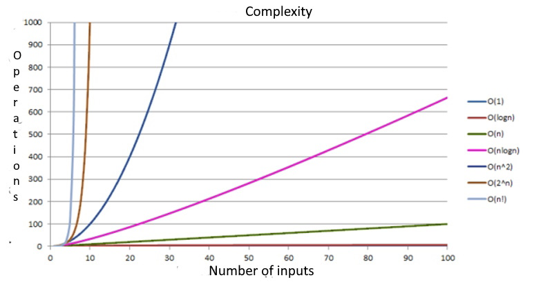
As shown in this table and graph, as the complexity of the function increases, the number of computations or the time required to perform the function can increase significantly. Next, the algorithms will be described with estimates of their complexity.
5.4. Space Complexity
Another characteristic of the computational complexity of algorithms is space complexity, estimated by the amount of memory required by the algorithm in its life cycle. This space consists of a fixed part and a variable part.
-
The fixed part is the space required to store simple variables and constants, as well as the program size, which is independent of the complexity of the task.
-
The variable part is the space required by variables whose size depends entirely on the size of the task. For example, recursion stack space, dynamic memory allocation, etc.
Space complexity is evaluated as O(1) if only the input data set is used. If the problem requires auxiliary memory of the same size as the input memory (memory to store the original array), then the space complexity is evaluated as O(n). In the case of a two-dimensional array or matrix, space complexity may be O(n²).
5.5. Algorithm Stability
It is especially important to know whether the algorithm used is stable, especially in situations where your data already has some order that you would like to preserve when sorting with a different key. For example, a spreadsheet has rows containing student data sorted by name by default. You would also like to sort it by class while maintaining the orderly order of names.
On the other hand, the stability of sorting does not matter when the sorting keys of objects in a collection are the objects themselves — arrays of integers or strings, for example — because we cannot determine the difference between duplicate keys.
5.6. Summary
This section established the theoretical and analytical foundations for evaluating algorithm performance and correctness, independently of specific hardware or JavaScript execution environments.
We explored the core principles of algorithmic efficiency: * Time and Space Complexity: Evaluating how execution time and auxiliary memory usage scale relative to the input size $n$. * Asymptotic Notations: Utilizing $\mathcal{O}$ (upper bound), $\Omega$ (lower bound), and $\Theta$ (tight bound) to classify algorithm growth rates (e.g., constant, logarithmic, linear, quadratic). * Abstract Machine Models: Analyzing algorithms via the RAM model to decouple performance metrics from compiler optimizations and environment overhead. * Algorithm Stability: Assessing whether an algorithm preserves the relative order of elements with equal keys, a critical property in multi-key sorting scenarios.
Understanding these analytical tools enables rigorous comparison between competing algorithmic solutions, ensuring optimal resource utilization in practical applications.